Logistic regression with JAX (and Flax)

JAX (and its higher level wrapper Flax) is a library for efficient numerical computation including automatic differentiation and JIT compilation.

This is an introduction to JAX and Flax using logistic regression as a simple example.

Logistic regression model specification

For a logistic regression model, we have

$l o g i t (p) = \log (\frac{p}{1 - p}) = β_{0} + β_{1} x_{1} + β_{2} x_{2} + \dots + β_{n} x_{n}$

(qlogis in R)

of which the inverse is the logistic function (plogis in R):

$p = \frac{1}{1 + e^{- (β_{0} + β_{1} x_{1} + β_{2} x_{2} + \dots + β_{n} x_{n})}}$

This formulation is nice because we can interpret the $β$ coefficients as the change in the log-odds of the outcome for a one unit increase in the corresponding feature.

However other choices are available e.g. using a probit model where we use the cumulative distribution function of the standard normal distribution instead of the logistic function.

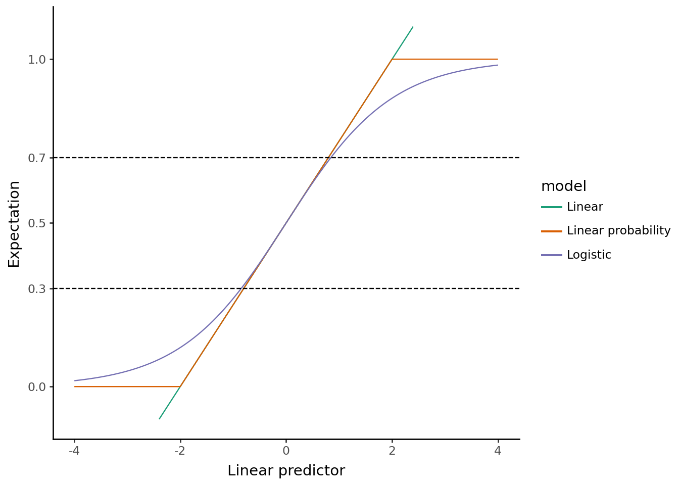
You can even use a gaussian GLM where we don’t transform the linear combination of the features at all.

Pros and Cons of the linear probability model

The gaussian GLM has the benefit that the coefficients are interpretable on the probability scale directly and it has a (fast to compute) closed form solution.

It also turns out to be unbiased and consistent for the average marginal effect.

However, it can predict probabilities outside of $(0, 1)$ , so it is only a good approximation for the conditional expectation when the probabilities are between 0.3 and 0.7:

Code

import numpy as np
import pandas as pd
import plotnine as pn
from scipy.stats import norm

n = 1000
xb = np.linspace(-4, 4, n)

# Define the models
linear = 0.25 * xb + 0.5
lpm = np.clip(linear, 0, 1)
logistic = 1 / (1 + np.exp(-xb))  # plogis - logistic/sigmoid function
probit = norm.cdf(xb)  # pnorm - probit link (Phi)
cloglog = 1 - np.exp(-np.exp(xb))  # complementary log-log link

df = pd.DataFrame({
    'xb': np.tile(xb, 3),
    'expectation': np.concatenate([logistic, linear, lpm]),
    'model': np.repeat(['Logistic', 'Linear', 'Linear probability'], n)
})

plot = (
    pn.ggplot(df, pn.aes(x='xb', y='expectation', color='model')) +
    pn.geom_line() +
    pn.scale_color_brewer(type='qual', palette='Dark2') +
    pn.theme_classic() +
    pn.scale_y_continuous(breaks=[0, 0.3, 0.5, 0.7, 1.0], limits=[-0.1, 1.1]) +
    pn.geom_hline(yintercept=0.3, linetype='dashed', color='black') +
    pn.geom_hline(yintercept=0.7, linetype='dashed', color='black') +
    pn.labs(
        x='Linear predictor',
        y='Expectation'
    )
)

plot.show()

/opt/hostedtoolcache/Python/3.12.12/x64/lib/python3.12/site-packages/plotnine/geoms/geom_path.py:100: PlotnineWarning: geom_path: Removed 200 rows containing missing values.

So we have a map between the linear combination of the features ( $X β$ ) and the probability of the outcome $p$ , but we still need to specify the distribution of the outcomes to get a full generative model.

Given we have outcomes $y \in {0, 1}$ , and assuming a conditional (on $x$ ) mean $p$ , the maximum entropy distribution is the Bernoulli distribution $P (y) = p^{y} (1 - p)^{1 - y}$

Which is a neat way to write:

$P (y) = {\begin{cases} p & if y = 1, \\ 1 - p & if y = 0. \end{cases}$

and so the full model is:

$y \sim B e r n o u l l i (p)$

$p = \frac{1}{1 + e^{- (β_{0} + β_{1} x_{1} + β_{2} x_{2} + \dots + β_{n} x_{n})}}$

Parameter estimation

To find the “best” $β$ coefficients (in the sense of maximizing the probability of the observed data) we can use maximum likelihood estimation.

For multiple independent observations $y_{i}$ , the likelihood is given by the product of the individual probabilities:

$L (p) = \prod_{i = 1}^{n} p_{i}^{y_{i}} (1 - p_{i})^{1 - y_{i}}$

We want to maximize this likelihood function which is equivalent to minimizing the negative log-likelihood function:

$J = - \frac{1}{n} \sum_{i = 1}^{n} [y_{i} \log (p_{i}) + (1 - y_{i}) \log (1 - p_{i})]$

aka the binary cross-entropy loss function.

JAX: autodiff for gradient descent

We can code both the data generation and loss function in JAX at a high level quite easily:

import jax
import jax.numpy as jnp
import numpy as np
import statsmodels.api as sm

def logistic(z):
    return 1 / (1 + jnp.exp(-z))

def predict(weights, bias, predictors):
    """ Probabilities of the positive class """
    return logistic(jnp.dot(predictors, weights) + bias)

def generate_data(num_samples = 100_000, seed = 42):
    rng = np.random.default_rng(seed)
    predictors = rng.standard_normal((num_samples, 2))
    true_weights = np.array([1.5, -0.8])
    true_bias = 0.3
    p = predict(true_weights, true_bias, predictors)
    y = rng.binomial(1, p)
    return predictors, y, true_weights, true_bias

def loss(weights, bias, predictors, targets):
    # while not the most numerically stable, 
    # this form more closely parallels the likelihood function above
    preds = predict(weights, bias, predictors)
    term_1 = targets * jnp.log(preds + 1e-15)
    term_2 = (1 - targets) * jnp.log(1 - preds + 1e-15)
    # jnp.mean = (1/n * sum)
    return -jnp.mean(term_1 + term_2)

To train this model in JAX we can use the automatic differentiation and use gradient descent:

grad_fn = jax.grad(loss, argnums=(0, 1))

@jax.jit
def update_step(weights, bias, predictors, targets, learning_rate):
    dw, db = grad_fn(weights, bias, predictors, targets)
    new_weights = weights - learning_rate * dw
    new_bias = bias - learning_rate * db
    return new_weights, new_bias

def train_model(X, y, key):
    w = jax.random.normal(key, shape=(2,))
    b = 0.0

    learning_rate = 0.1
    for i in range(501):
        w, b = update_step(w, b, X, y, learning_rate)
        if i % 100 == 0:
            current_loss = loss(w, b, X, y)
            print(f"Epoch {i}: Loss = {current_loss:.4f}")

    print(f"Learned Weights: {w}")
    print(f"Learned Bias: {b:.4f}")

X, y, true_w, true_b = generate_data()
key = jax.random.PRNGKey(0)
train_model(X, y, key)
print(f"\nTrue Weights: {true_w}")
print(f"True Bias: {true_b}")

Epoch 0: Loss = 1.1145
Epoch 100: Loss = 0.5188
Epoch 200: Loss = 0.4960
Epoch 300: Loss = 0.4951
Epoch 400: Loss = 0.4950
Epoch 500: Loss = 0.4950
Learned Weights: [ 1.5045096  -0.79790395]
Learned Bias: 0.2995

True Weights: [ 1.5 -0.8]
True Bias: 0.3

While stochastic gradient descent is often used, our dataset is small enough that we can use the full gradient.

Let’s compare to the statsmodels implementation:

def train_model_smf(X, y):
    model = sm.Logit(y, sm.add_constant(X)).fit()
    print(model.summary())

train_model_smf(X, y)

print(f"\nTrue Weights: {true_w}")
print(f"True Bias: {true_b}")

Optimization terminated successfully.
         Current function value: 0.494975
         Iterations 6
                           Logit Regression Results                           
==============================================================================
Dep. Variable:                      y   No. Observations:               100000
Model:                          Logit   Df Residuals:                    99997
Method:                           MLE   Df Model:                            2
Date:                Tue, 10 Feb 2026   Pseudo R-squ.:                  0.2810
Time:                        00:50:36   Log-Likelihood:                -49498.
converged:                       True   LL-Null:                       -68842.
Covariance Type:            nonrobust   LLR p-value:                     0.000
==============================================================================
                 coef    std err          z      P>|z|      [0.025      0.975]
------------------------------------------------------------------------------
const          0.3012      0.008     38.199      0.000       0.286       0.317
x1             1.5128      0.011    140.758      0.000       1.492       1.534
x2            -0.8028      0.009    -92.580      0.000      -0.820      -0.786
==============================================================================

True Weights: [ 1.5 -0.8]
True Bias: 0.3

It’s more succinct, and you also get standard errors (and p-values), however the JAX implementation is more flexible. For example we could easily switch to a probit model by just changing the sigmoid function to the CDF of the standard normal distribution:

def predict_probit(weights, bias, predictors):
    """ Probabilities of the positive class """
    return norm.cdf(jnp.dot(predictors, weights) + bias)

or add regularisation:

def loss_ridge(weights, bias, predictors, targets, lambda_val):
    return loss(weights, bias, predictors, targets) + lambda_val * jnp.mean(weights**2)

Flax: a higher level API

While we used standard gradient descent above, with Flax we can use more sophisticated optimisers like Adam which adjust the learning rate for example using momentum.

import flax.linen as nn
from flax.training import train_state
import optax

class LogisticRegression(nn.Module):
    @nn.compact
    def __call__(self, x):
        # A simple linear layer with 1 output (the logit)
        return nn.Dense(features=1, use_bias=True)(x)


def loss_fn(params, apply_fn, X, y):
    logits = apply_fn({'params': params}, X).squeeze()
    return optax.sigmoid_binary_cross_entropy(logits, y).mean()


@jax.jit
def train_step_adam(state, X, y):
    loss_val, grads = jax.value_and_grad(loss_fn)(state.params, state.apply_fn, X, y)
    updates, new_opt_state = state.tx.update(grads, state.opt_state, state.params)
    new_params = optax.apply_updates(state.params, updates)
    return state.replace(params=new_params, opt_state=new_opt_state), loss_val


def train_model(X, y, key):
    model = LogisticRegression()
    variables = model.init(key, jnp.ones((1, 2)))
    tx_adam = optax.adam(learning_rate=0.1)
    state_adam = train_state.TrainState.create(
        apply_fn=model.apply,
        params=variables['params'],
        tx=tx_adam
    )
    for i in range(101):
        state_adam, loss = train_step_adam(state_adam, X, y)
        if i % 10 == 0:
            print(f"Epoch {i}: Loss = {loss:.4f}")

    print("Learned Weights: ")
    print(state_adam.params)

train_model(X, y, key)
print(f"\nTrue Weights: {true_w}")
print(f"True Bias: {true_b}")

Epoch 0: Loss = 1.2306
Epoch 10: Loss = 0.7032
Epoch 20: Loss = 0.5401
Epoch 30: Loss = 0.4987
Epoch 40: Loss = 0.4956
Epoch 50: Loss = 0.4960
Epoch 60: Loss = 0.4958
Epoch 70: Loss = 0.4955
Epoch 80: Loss = 0.4951
Epoch 90: Loss = 0.4950
Epoch 100: Loss = 0.4950
Learned Weights: 
{'Dense_0': {'bias': Array([0.30004427], dtype=float32), 'kernel': Array([[ 1.5121937 ],
       [-0.80526525]], dtype=float32)}}

True Weights: [ 1.5 -0.8]
True Bias: 0.3

We can also use LBFG-S, which is a second order optimiser (it uses the Hessian - the matrix of second derivatives). So while each update is more expensive, it doesn’t require as many iterations:

@jax.jit
def train_step_lbfgs(state, X, y):
    loss_val, grads = jax.value_and_grad(loss_fn)(state.params, state.apply_fn, X, y)
    
    # L-BFGS needs value and grad passed to update
    updates, new_opt_state = state.tx.update(
        grads, state.opt_state, state.params,
        value=loss_val, grad=grads, 
        value_fn=lambda p: loss_fn(p, state.apply_fn, X, y)
    )
    new_params = optax.apply_updates(state.params, updates)
    return state.replace(params=new_params, opt_state=new_opt_state), loss_val

def train_model_lbfgs(X, y, key):
    model = LogisticRegression()
    variables = model.init(key, jnp.ones((1, 2)))
    tx_lbfgs = optax.lbfgs(memory_size=10)
    state_lbfgs = train_state.TrainState.create(
        apply_fn=model.apply,
        params=variables['params'],
        tx=tx_lbfgs
    )
    
    for i in range(6):
        state_lbfgs, loss = train_step_lbfgs(state_lbfgs, X, y)
        print(f"Epoch {i}: Loss = {loss:.4f}")  

    print("Learnt weights:")
    print(state_lbfgs.params)

train_model_lbfgs(X, y, key)
print(f"\nTrue Weights: {true_w}")
print(f"True Bias: {true_b}")

Epoch 0: Loss = 1.2306
Epoch 1: Loss = 0.9719
Epoch 2: Loss = 0.5134
Epoch 3: Loss = 0.5010
Epoch 4: Loss = 0.4954
Epoch 5: Loss = 0.4950
Learnt weights:
{'Dense_0': {'bias': Array([0.30116275], dtype=float32), 'kernel': Array([[ 1.5125961],
       [-0.8026858]], dtype=float32)}}

True Weights: [ 1.5 -0.8]
True Bias: 0.3

The real power here comes from the flexibility to train almost arbitrary models. A logistic regression is just a single layer neural network, but we can easily add more layers:

class LogisticRegressionNN(nn.Module):
    @nn.compact
    def __call__(self, x):
        # A simple neural network with 1 hidden layer and 1 output (the logit)
        x = nn.Dense(features=10, use_bias=True)(x)
        x = nn.relu(x)
        return nn.Dense(features=1, use_bias=True)(x)


def train_model_nn(X, y, key):
    model = LogisticRegressionNN()
    variables = model.init(key, jnp.ones((1, 2)))
    tx_adam = optax.adam(learning_rate=0.1)
    state_adam = train_state.TrainState.create(
        apply_fn=model.apply,
        params=variables['params'],
        tx=tx_adam
    )
    for i in range(101):
        state_adam, loss = train_step_adam(state_adam, X, y)
        if i % 10 == 0:
            print(f"Epoch {i}: Loss = {loss:.4f}")

train_model_nn(X, y, key)

Epoch 0: Loss = 0.6905
Epoch 10: Loss = 0.5051
Epoch 20: Loss = 0.4985
Epoch 30: Loss = 0.4972
Epoch 40: Loss = 0.4964
Epoch 50: Loss = 0.4956
Epoch 60: Loss = 0.4952
Epoch 70: Loss = 0.4951
Epoch 80: Loss = 0.4950
Epoch 90: Loss = 0.4950
Epoch 100: Loss = 0.4950

While in this case we generated data from the logistic model so we don’t improve much on the loss. For more complicated data generating processes this general model training procedure is quite powerful.