Why coord_serial instead of standard faceting?
One way to plot genomic data in ggplot2 is using facet_grid(). However, for complex plots like a Manhattan plot, this approach leads to a fragmented visualization and layering issues.
The facet_grid Approach
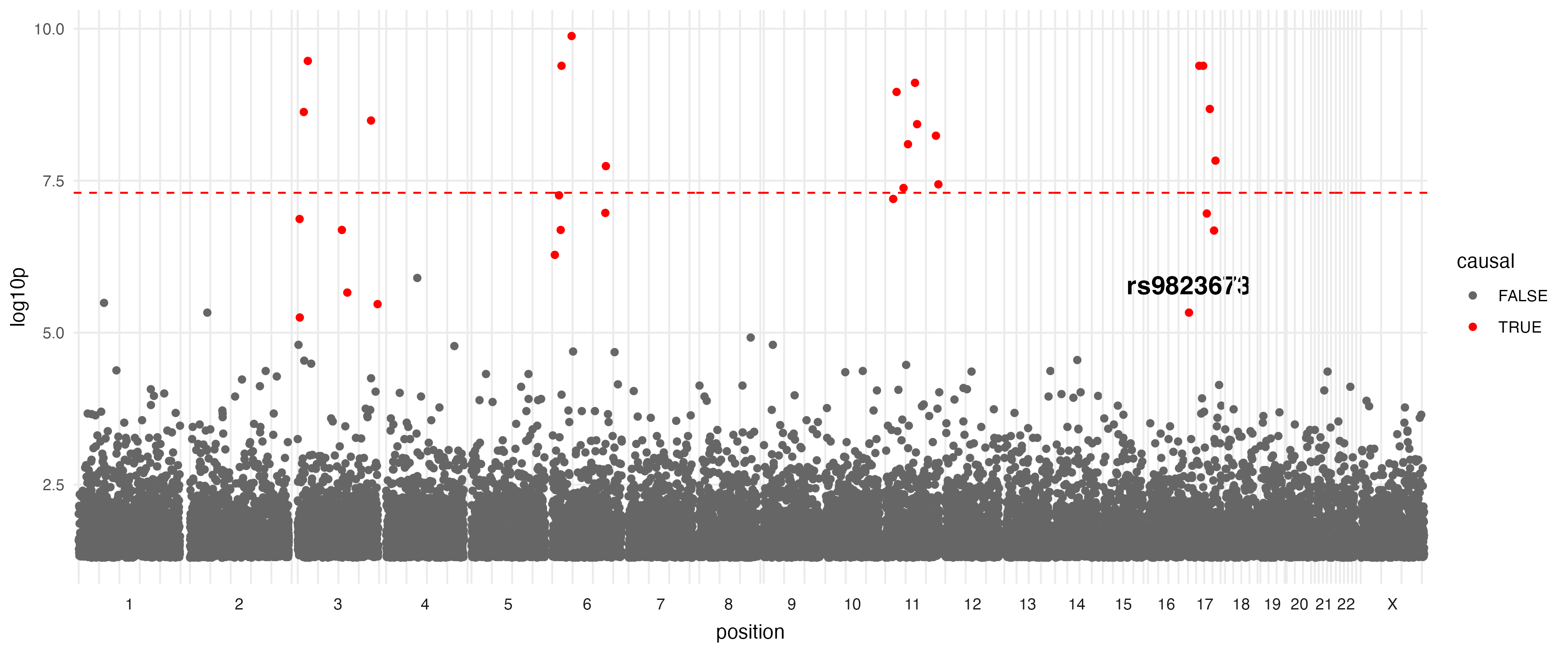
To get proportional widths for chromosomes, you must use facet_grid(. ~ chrom, scales = "free_x", space = "free_x"). Even with panel.spacing = unit(0, "lines"), there is not consistent spacing between chromosomes and even with coord_cartesian(clip = "off"), labels don’t span multiple regions cleanly.
library(ggplot2)
library(coord.serial)

target_hit <- simulated_gwas[simulated_gwas$chrom == "17" & simulated_gwas$causal, ][1, ]
target_hit$label <- "rs9823673"

ggplot(simulated_gwas, aes(x = position, y = log10p)) +
    geom_point(aes(color = causal)) +
    geom_text(data = target_hit, aes(label = label), vjust = -1) +
    geom_hline(yintercept = -log10(5e-8), color = "red", linetype = "dashed") +
    facet_grid(. ~ chrom, scales = "free_x", space = "free_x", switch = "x") +
    coord_cartesian(clip = "off") + # Attempt to prevent label clipping
    theme_minimal() +
    theme(
        panel.spacing = unit(0, "lines"),
        strip.placement = "outside",
        panel.grid.minor = element_blank()
    )
The coord_serial Approach
p <- ggplot(simulated_gwas, aes(x = position, y = log10p, domain = chrom, color = causal)) +
    geom_point() +
    geom_text(data = target_hit, aes(label = label), vjust = -1) +
    geom_hline(yintercept = -log10(5e-8), color = "red", linetype = "dashed") +
    coord_serial() +
    theme_minimal()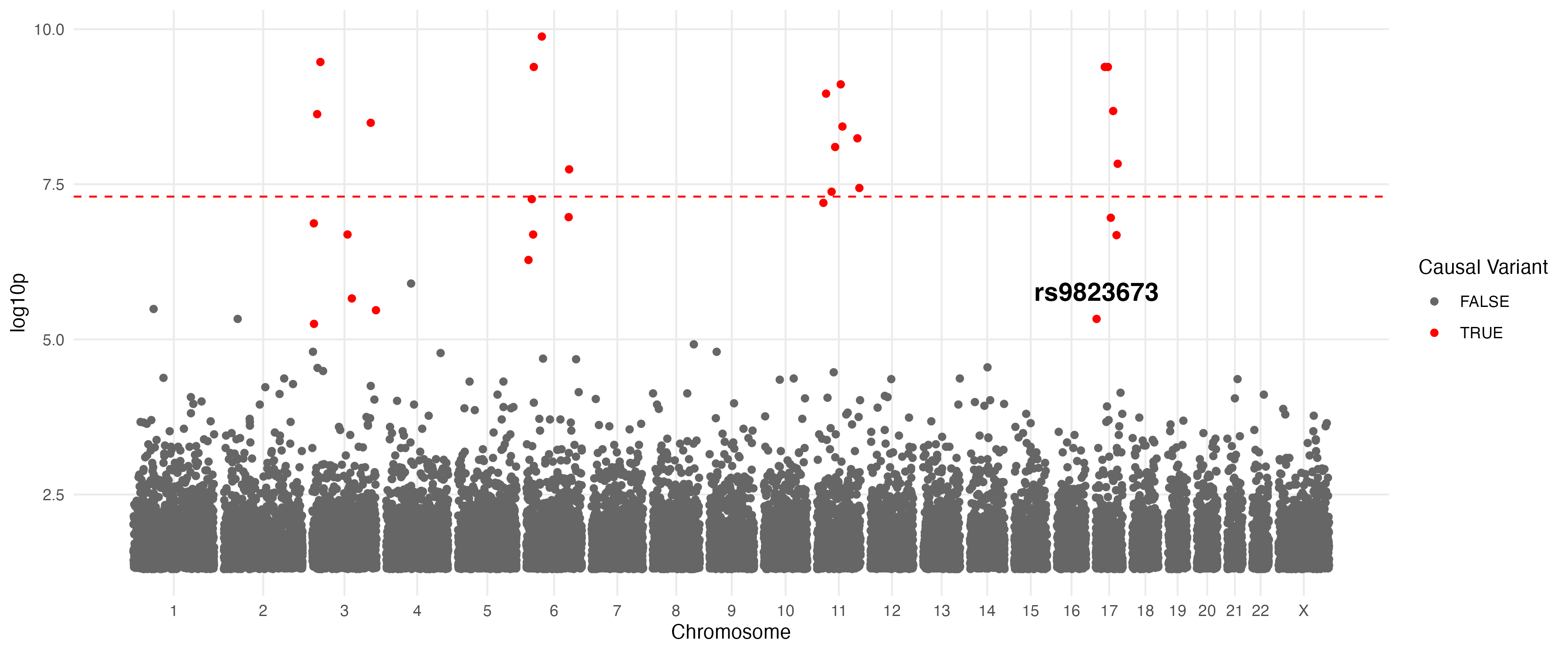
Key Advantages of coord_serial()
1. Unified Canvas (Zero Artifacts)
In facet_grid, even if you use clip = "off", labels that cross into adjacent panels face z-index issues. Because facets are drawn one by one, a label from Chromosome 17 is drawn behind the background and grid lines of Chromosome 18 (\(rs9...\) in the plot above).
In coord_serial(), the entire plot is a single panel, so labels and lines span boundaries perfectly.
2. Seamless Axis
Because coord_serial() maps multiple domains to a single continuous x-axis, the axis line is unbroken. Faceting creates a “comb” effect with 23 independent axes that are difficult to style consistently.
3. Logical Coordinates
You can add annotations (like geom_rect or geom_segment) across multiple chromosomes using a single x-scale. With faceting, you are logically restricted to one panel at a time.
4. Minimal Code
coord_serial() automatically handles proportional scaling and domain gaps. You don’t need to remember complex facet_grid arguments like scales = "free_x" and space = "free_x".