A mixture of gaussian distibutions can be used to approximate a different non gaussian distribution. For example the hights of a population may be non-normal, but are well approximated by a mixture of two normal distributions which could represent the hights of sex. Sometimes you might have multiple datasets (or a single dataset segmented by some parameter) and you want to fit a gaussian mixture model to all data sets at once but for there to be some components which are shared across these data sets.
This is a vignette for an R package I created called comixr.
library(comixr)
library(data.table)
Simple Example
Let’s simulate two datasets, each with a common density at ~5 and with some noise component with mean and variance unique to each dataset.
input <- rbind(data.table(vals = rnorm(2000, mean = 5.0, sd = 0.75), seg = 1),
               data.table(vals = rnorm(1000, mean = 0.5, sd = 1.0), seg = 1),
              data.table(vals = rnorm(2000, mean = 5.5, sd = 0.75), seg = 2),
              data.table(vals = rnorm(2000, mean = 4.0, sd = 3.0), seg = 2))
We need to specify our initial components for each component type:
initial.parameters <- data.table(
  w = 0.5,
  mean = c(6,4),
  variance = 1,
  component.type = c("common","specific"))

initial.parameters

##      w mean variance component.type
## 1: 0.5    6        1         common
## 2: 0.5    4        1       specific
Now we can fit the model:
output <- fit_comixture(input, initial.parameters)

## [1] "2 segments, each with 1 common component(s), and 1 specific component(s)"
## [1] "Iteration: 1"
## [1] "Iteration: 2"
## [1] "Iteration: 3"
## [1] "Iteration: 4"
## [1] "Iteration: 5"
## [1] "Iteration: 6"
## [1] "Iteration: 7"
## [1] "Iteration: 8"
## [1] "Iteration: 9"
## [1] "Iteration: 10"
## [1] "Iteration: 11"
## [1] "Iteration: 12"
## [1] "Iteration: 13"
## [1] "Iteration: 14"
## [1] "Iteration: 15"
## [1] "Iteration: 16"
## [1] "Finished after 16 iterations (0.1 seconds)"
And plot the results:
plot_comixture(input, output)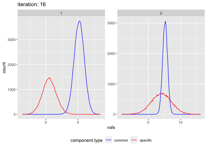
plot_comixture(input, output, type = "density")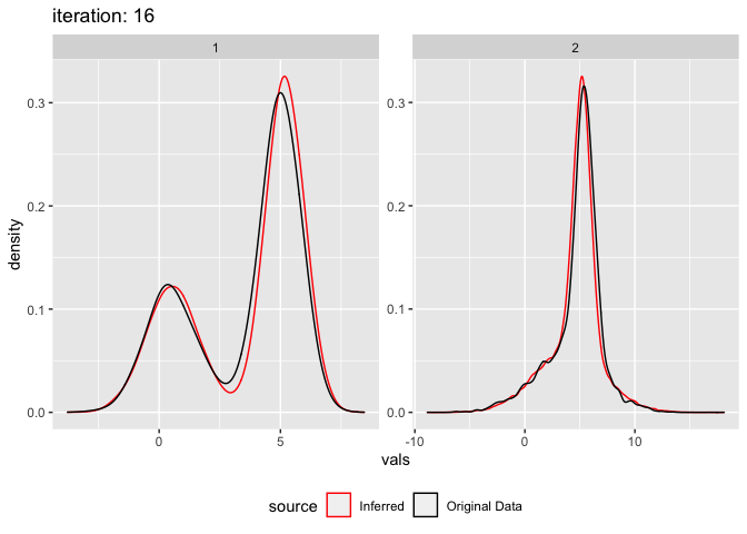
Multiple common and specific components
Lets simulate some example data, two data sets, each with four components, two of which are shared across the data sets and two of which are unique to the data set.
test.data.basic <- rbind(
# Common components
            data.table(comp = "A", vals = rnorm(2000, mean = 5, sd = 0.5), seg = 1),
            data.table(comp = "A", vals = rnorm(2000, mean = 5, sd = 0.5), seg = 2),

            data.table(comp = "B", vals = rnorm(1500, mean = 9, sd = 0.5), seg = 1),
            data.table(comp = "B", vals = rnorm(1500, mean = 9, sd = 0.5), seg = 2),

# Unique components
            data.table(comp = "C", vals = rnorm(3000, mean = -1, sd = 0.5), seg = 1),
            data.table(comp = "D", vals = rnorm(2000, mean = 3, sd = 0.5), seg = 2),

            data.table(comp = "E", vals = rnorm(1500, mean = 10, sd = 0.5), seg = 1),
            data.table(comp = "F", vals = rnorm(1500, mean = 13, sd = 0.5), seg = 2)
            )

knitr::kable(head(test.data.basic, 5))| comp | vals | seg |
|---|---|---|
| A | 5.314453 | 1 |
| A | 5.772871 | 1 |
| A | 4.909807 | 1 |
| A | 4.980014 | 1 |
| A | 4.325934 | 1 |
Let’s visualise the distribution of the two data sets broken down by component
library(ggplot2)

## Warning: package 'ggplot2' was built under R version 3.6.2

ggplot(test.data.basic, aes(vals, colour = comp)) +
  geom_freqpoly(binwidth = 0.1) +
  facet_wrap(~seg, nrow = 2)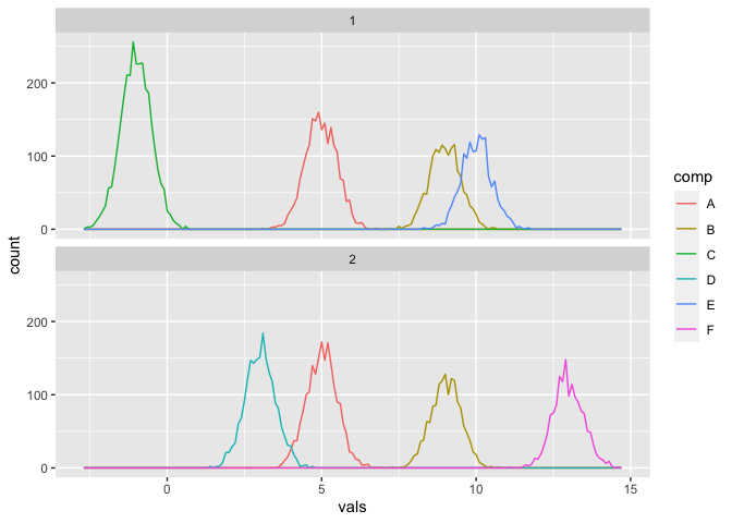
Fitting the model
To fit a shared gaussian mixture model to this data we need to specify the number of components in the model and the initial parameters for each component. w is the mixing weight of each component, mu the mean, and variance (σ2). By default comixr uses the EM algorithm, but it can also use the VB.
initial.parameters.basic.vb.1 <- data.table(
  mean = c(6,7,0.6,15),
  nu = c(0.1),
  scale = c(2^3),
  shape = c(2^(-4)),
  component.type = c("common","common","specific","specific"))

initial.parameters.basic.vb.1

##    mean  nu scale  shape component.type
## 1:  6.0 0.1     8 0.0625         common
## 2:  7.0 0.1     8 0.0625         common
## 3:  0.6 0.1     8 0.0625       specific
## 4: 15.0 0.1     8 0.0625       specific
To fit the model pass the data (without the component labels), the initial rho, and the other componentwise initial parameters to the fit_comixture() function.
output.test.basic.vb.1 <- fit_comixture(test.data.basic[,.(vals,seg)], initial.parameters.basic.vb.1, max.iterations = 60, algorithm = "VB", quiet = TRUE)

## [1] "2 segments, each with 2 common component(s), and 2 specific component(s)"
## [1] "Finished after 60 iterations (0.6 seconds)"
We can then visualise the result using the plot_comixture() function.
plot_comixture(test.data.basic, output.test.basic.vb.1)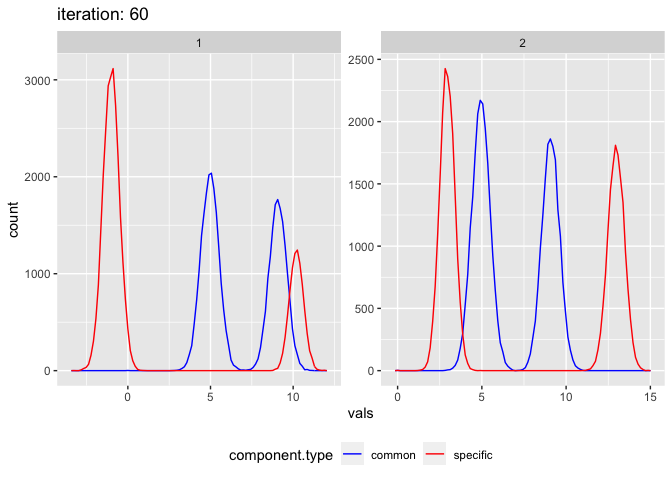
plot_comixture(test.data.basic, output.test.basic.vb.1, type = "density")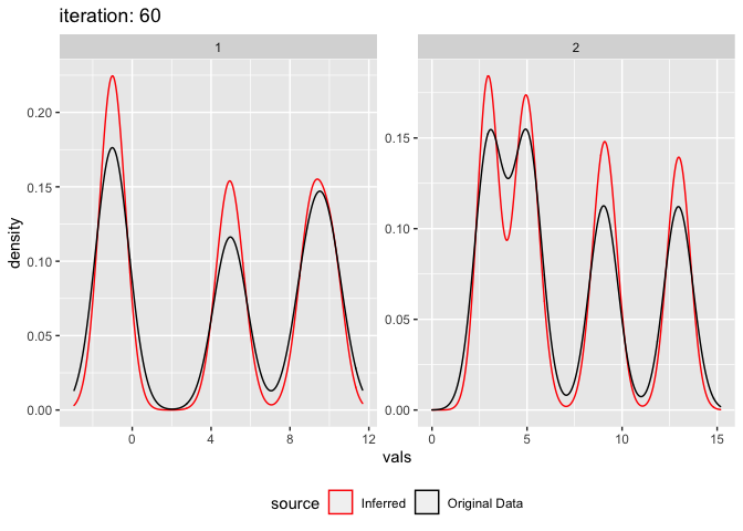
plot_comixture(test.data.basic, output.test.basic.vb.1, type = "QQ")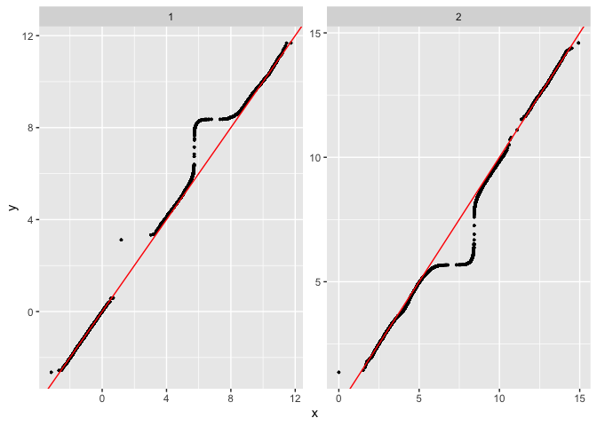
This is also a good case to demonstrate the failure of this algorithm. Depending on the inital means the method can get stuck in a local maxima. E.g. change the mean 0.6 to 0.4.
initial.parameters.basic.vb.2 <- data.table(
  mean = c(6,7,0.4,15),
  nu = c(0.1),
  scale = c(2^3),
  shape = c(2^(-4)),
  component.type = c("common","common","specific","specific"))

output.test.basic.vb.2 <- fit_comixture(test.data.basic[,.(vals,seg)], initial.parameters.basic.vb.2, max.iterations = 60, algorithm = "VB", quiet = TRUE)

## [1] "2 segments, each with 2 common component(s), and 2 specific component(s)"
## [1] "Finished after 60 iterations (0.7 seconds)"

plot_comixture(test.data.basic, output.test.basic.vb.2)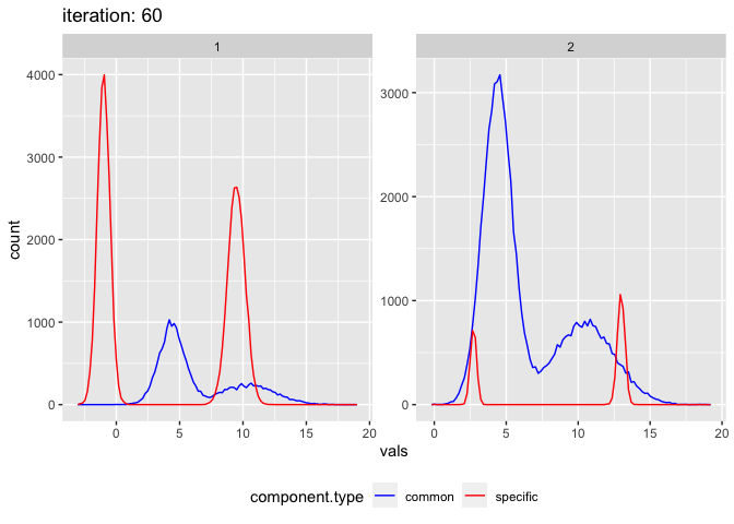
plot_comixture(test.data.basic, output.test.basic.vb.2, type = "density")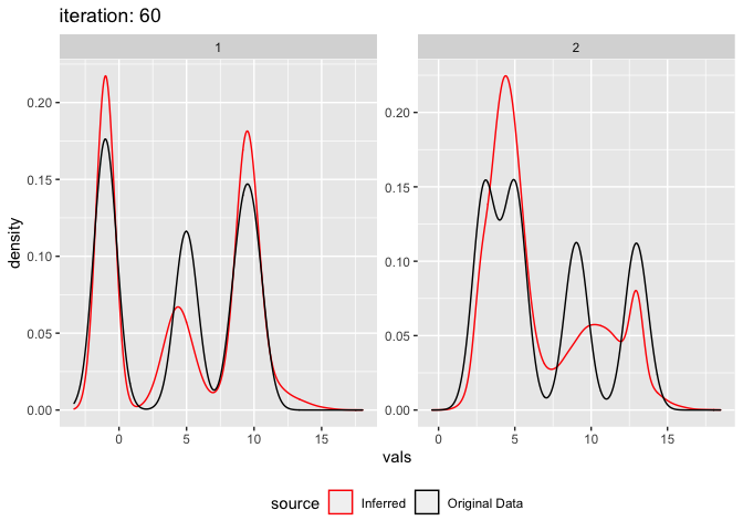
plot_comixture(test.data.basic, output.test.basic.vb.2, type = "QQ")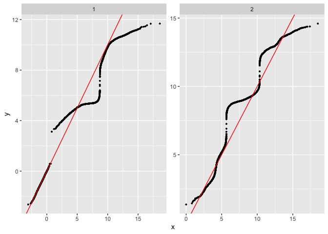
If one of the input parameters is completely wrong e.g. if we change mean of 15 to 150, an error will be produced.
initial.parameters.basic.vb.3 <- data.table(
  mean = c(6,7,0.6,150),
  nu = c(0.1),
  scale = c(2^3),
  shape = c(2^(-4)),
  component.type = c("common","common","specific","specific"))

output.test.basic.vb.3 <- fit_comixture(test.data.basic[,.(vals,seg)], initial.parameters.basic.vb.3, max.iterations = 60, algorithm = "VB")

## [1] "2 segments, each with 2 common component(s), and 2 specific component(s)"

## Error in VB(segment.indicies, read.count, rho, com.param, n.specific.components, : sum(specific_parameters$mix_weights == 0) == 0 is not TRUE
Non gaussian underlying data
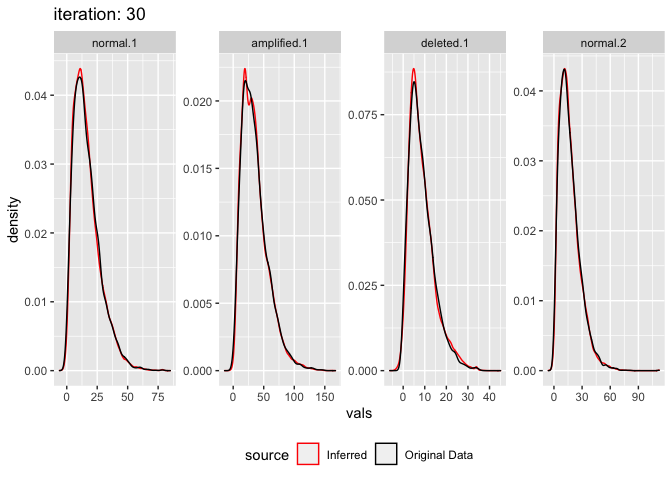
The model can also be fitted to data which isn’t actually made from multiple gaussians at all. Simulate realistic read count data using negative binomial, 4 segments, 2 normal, 1 amp, 1 del. Parameters from real data
test.data.realistic <- rbind(
  data.table(comp = "A", vals = rnbinom(5000, size=2.7, mu = 16.5), seg = "normal.1"),
  data.table(comp = "A", vals = rnbinom(5000, size=3, mu = 36), seg = "amplified.1"),
  data.table(comp = "A", vals = rnbinom(5000, size=2.9, mu = 8.4), seg = "deleted.1"),
  data.table(comp = "A", vals = rnbinom(5000, size=2.7, mu = 16.5), seg = "normal.2"))

initial.parameters.realistic <- data.table(
  w = c(0.5),
  mean = c(3,4,6,8,10,13,17,20,25,40,50,100,1,2),
  variance = c(8^2),
  component.type = c(rep("common",9),rep("specific",5)))

output.realistic <- fit_comixture(test.data.realistic[,.(vals,seg)], initial.parameters.realistic, quiet = TRUE)

## [1] "4 segments, each with 9 common component(s), and 5 specific component(s)"
## [1] "Finished after 30 iterations (1.4 seconds)"

plot_comixture(test.data.realistic, output.realistic)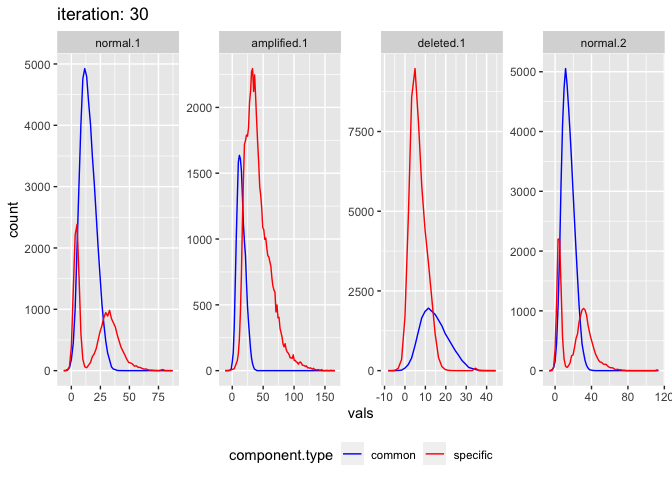
plot_comixture(test.data.realistic, output.realistic, type = "density")