| mean | sd | hdi_3% | hdi_97% | mcse_mean | mcse_sd | ess_bulk | ess_tail | r_hat | |
|---|---|---|---|---|---|---|---|---|---|
| mu_log_phase | 1.219 | 0.147 | 0.945 | 1.492 | 0.005 | 0.003 | 1023.0 | 1619.0 | 1.0 |
| Intercept | 0.703 | 0.127 | 0.459 | 0.941 | 0.003 | 0.002 | 1389.0 | 1751.0 | 1.0 |
| sigma_log_phase | 0.678 | 0.137 | 0.436 | 0.938 | 0.004 | 0.003 | 1368.0 | 1944.0 | 1.0 |
| sigma_level | 0.350 | 0.011 | 0.328 | 0.371 | 0.000 | 0.000 | 1295.0 | 1698.0 | 1.0 |
| alpha | 79.704 | 14.515 | 54.566 | 107.809 | 0.256 | 0.279 | 3331.0 | 2378.0 | 1.0 |
| mean_phase_effect | 3.420 | 0.498 | 2.574 | 4.445 | 0.016 | 0.009 | 1023.0 | 1619.0 | 1.0 |
I have a Blueair Blue 3410 Air Purifier, which the manufacturer claims can “remove more than 99% particles”.
But how effective is it really? The quoted effectiveness and CADR (Clean Air Delivery Rate) is determined in highly controlled conditions in a sealed room, using the fastest fan speed. In reality it’s too loud to use the fastest fan speed all the time, sometimes I will open my windows, and perhaps the air quality where I live doesn’t require purification in the first place.
So I ran my own experiment to determine the real world effectiveness of my air purifier.
The basic idea is that some days I will leave the air purifier turned on, and some days I’ll leave it off, all while measuring the pollution level in my apartment (using a Quingping air monitor lite) so I can compare if the pollution is meaningfully lower when the air purifier is turned on.
Single case experimental designs
This type of experiment is called an N-of-1 trial, and is a type of single-case (experimental) design (SCD/SCED). In order for this type of experiment to be valid, the intervention (in this case turning the air purifier on or off) must not have long lasting effects i.e. when the intervention is removed the state goes back to baseline. For example administering a vaccine permanently changes the immune system, so you would instead need to use a randomised controlled trial (RCT) to determine its causal impact.
The RCT design is gold standard for determining causal effects, but if you can make the assumption that the intervention does not have long lasting effects, then an N-of-1 trial can be more efficient because it controls for the within-subject variability – each person is their own control.
TipSample size for a paired vs two sample t-test
A paired test may require four times fewer individuals than a two sample test to achieve the same statistical power to determine a difference.
A paired test is equivalent to a single group test performed on the differences.
A useful rule of thumb (Lehr’s Equation) is that the sample size required per group for a two sample t-test is:
n = \frac{16}{\Delta^2}
Where \Delta is the standardised difference:
\Delta = \frac{\mu_0 - \mu_1}{\sigma}
where \mu_0 and \mu_1 is the original and new mean respectively and \sigma is the standard deviation within a group (assumed to be equal in both).
In the one-sample or paired case the numerator becomes 8 instead of 16. This means you need half as many individuals per group in a one-sample or paired test. Since there’s only one group, in total that’s a 4-fold reduction in number of individuals. Of course, in the paired case you still need two observations per individual. So if it’s the observations that are expensive rather than individuals per se, then it’s not quite as beneficial.
This assumes that the standardised difference \Delta is the same, but in the paired case, it’s the standard devidation between the differences, which depends on the correlation between the pairs:
\sigma_d = \sigma \sqrt{2(1-\rho)}
when \rho=0.5 then \sigma_d = \sigma, but if \rho<0.5 then the fold reduction in sample size for a paired test is less (2 fold at \rho=0) and would be greater for more highly correlated samples.
Where does this rule of thumb come from?
n = \frac{2(Z_{1 - \alpha/2} + Z_{1-\beta})^2}{\Delta^2}
where
Z_{1 - \alpha/2} = 1.96
and
Z_{1-\beta} = 0.84
so the numerator becomes 15.68 ~= 16.
How accurate is it?
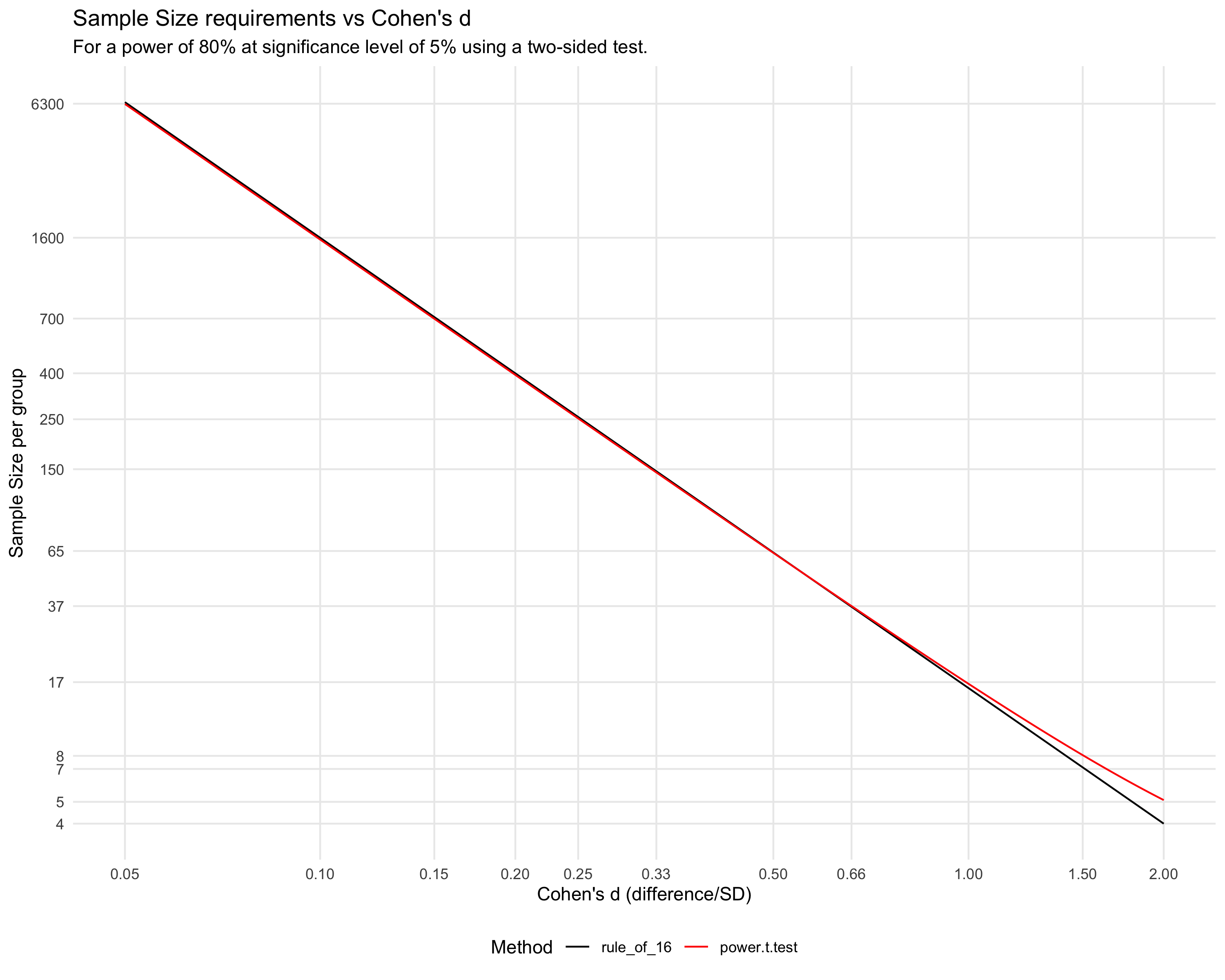
As the graph shows, this rule of thumb works very well, only deviating by a small relative amount for the smallest sample sizes.
Another benefit of a SCED is that it allows you to measure the effect of the intervention in your specific context (e.g. individual, location), which is often more relevant than the average effect across a group, as measured in a RCT.
Even if the state of interest does not return to baseline instantly, we can build in a ‘washout’ period to allow the air quality to return to baseline before measuring again.
This type of experiment also relies on the assumption that the change in the outcome is due to the intervention, and not some other factor that happened to occur at around the same time. In order to minimise this risk, the intervention can be repeated. The design of this repeated intervention is called a phase pattern. For example, a common phase pattern is ABAB, where A is the baseline and B is the intervention. Or more generally AB^k where k is the number of times this pattern is repeated. Ideally both the pattern and the time period of each phase should be randomised to avoid confounding with some other factor that has a similar periodicity. For example, perhaps a nearby farmer sprays pesticides every other day - if my period is 1 day in a AB^k design my intervention will be confounded with the pesticide spraying.
There are ways to potentially use a SCED even if the treatment is more permanent - for example if the treatment is a drug that has a long lasting effect, you can use a multiple baseline design, where you have multiple subjects and the intervention timing is randomised/staggered such that it’s less likely to be confounded with some other factor.
Result: 90% reduction in PM2.5 exposure
My study was a simple (AB)^k design with 35 repeats of each phase (k=35), where each phase was 1 day long, including a 3 hour washout period between the phases. As I was manually switching the purifier on and off, I was not blinded to the intervention. Though ideally this would have been randomised through an automated system.
Let’s look at the overall distribution of the PM2.5 levels when the purifier was on vs off.
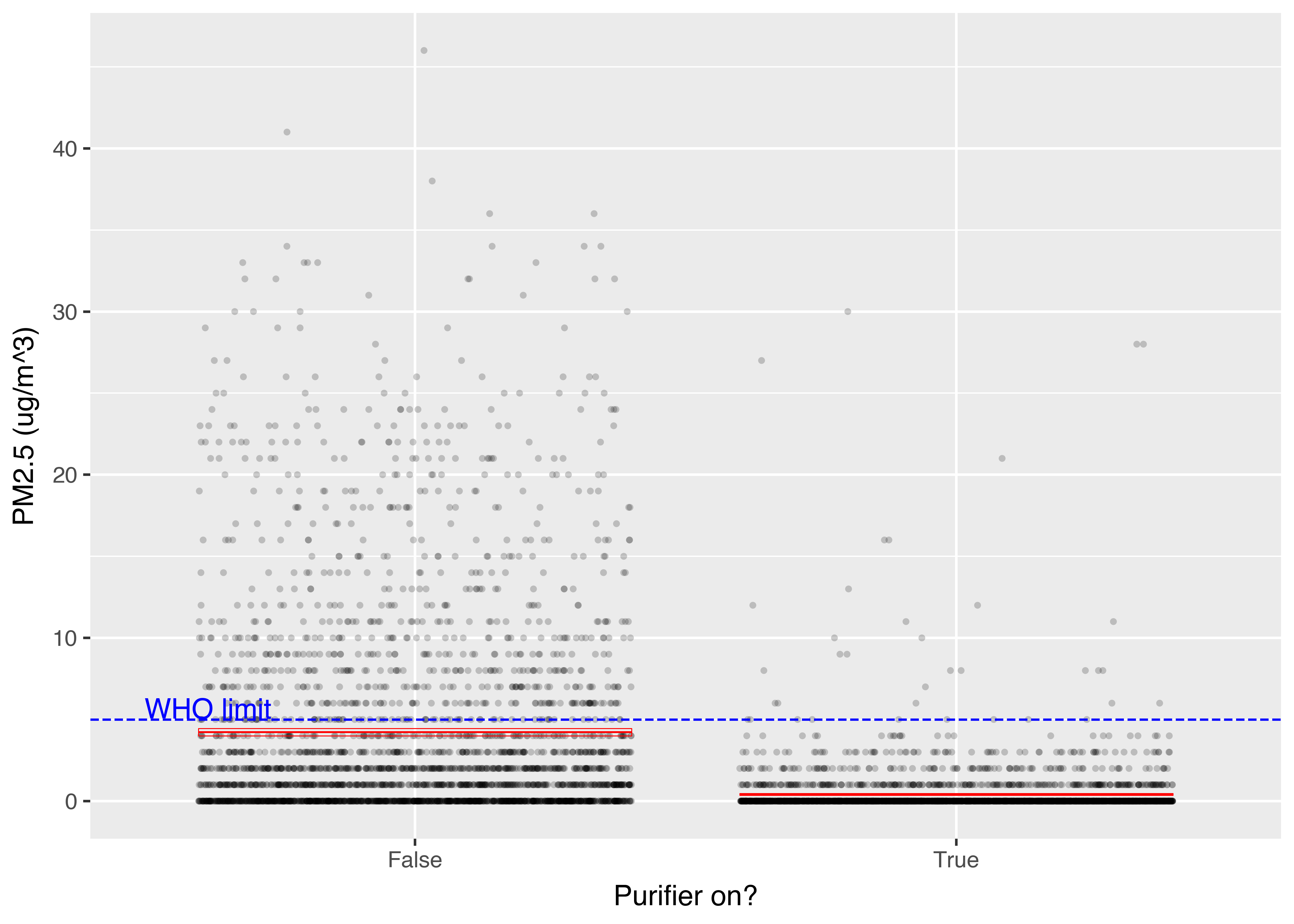
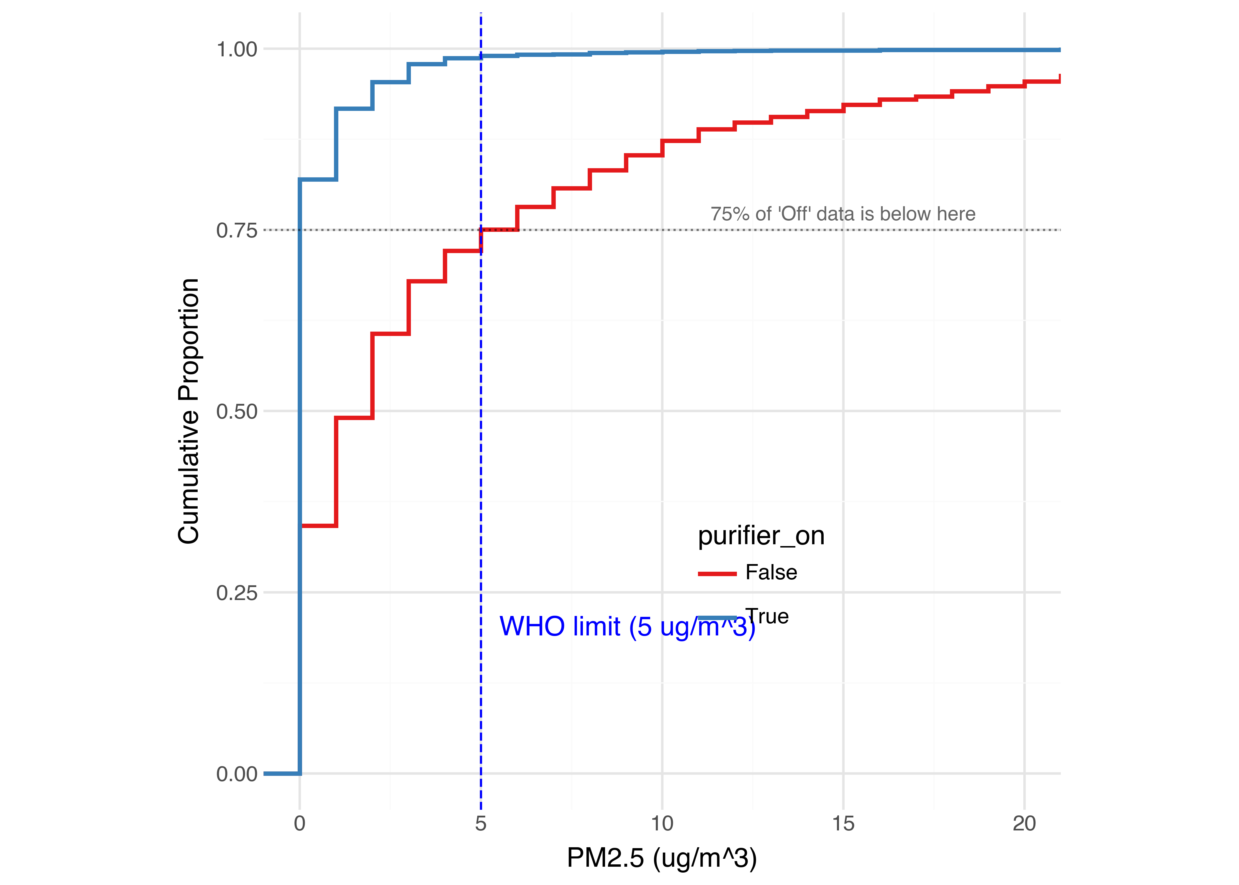
The mean PM2.5 level was 4.22 ug/m^3 when the purifier was off, and 0.41 ug/m^3 when it was on - a reduction of 90.3%. For comparison, the World Health Organisation (WHO) guidelines recommend a PM2.5 limit of 5 ug/m^3. Without the purifier, 24.9% of the measurements exceeded this limit; with the purifier, only 0.98% did (a 96% reduction).
This is a bit easier to see on the cumulative distribution graph. When the purifier is on, the distribution is shifted significantly to the left.
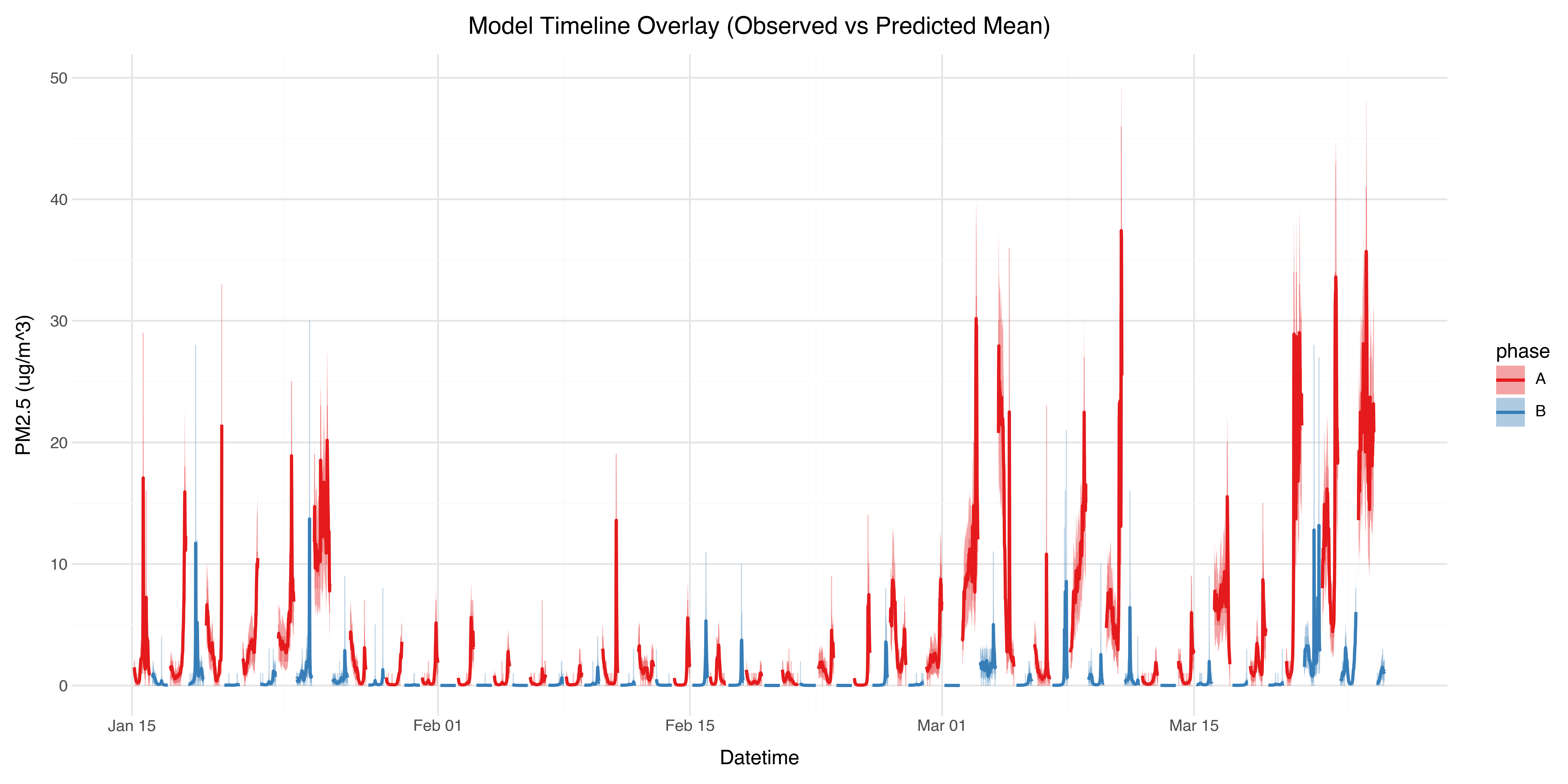
We can look at the levels over time to check for long term trends and other factors that might be confounding the results.
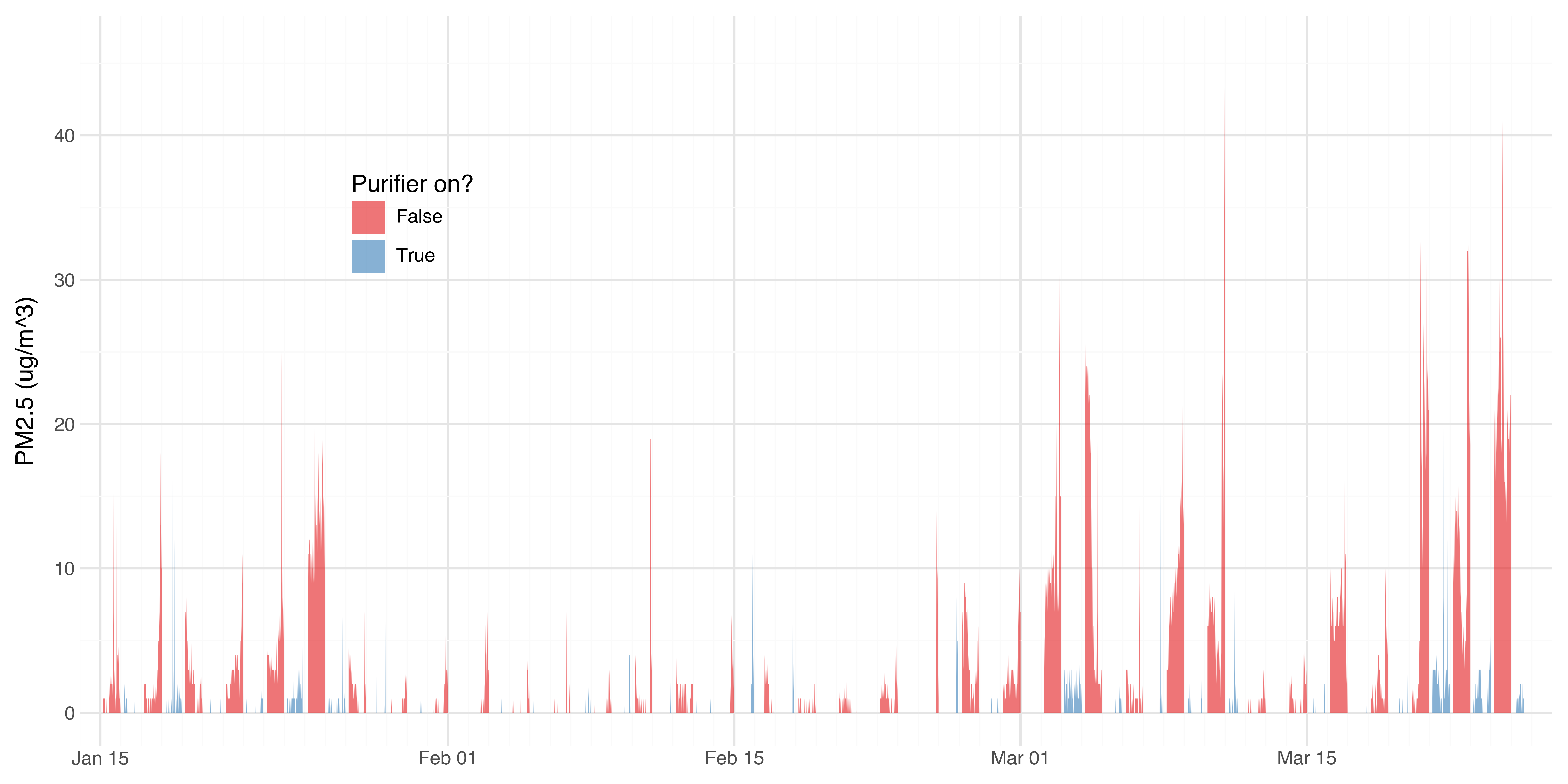
In February there wasn’t as much of a difference due to lower pollution levels to start with. So ideally the experiment should be run over an even longer time period to average out low frequency fluctuations in outside air quality.
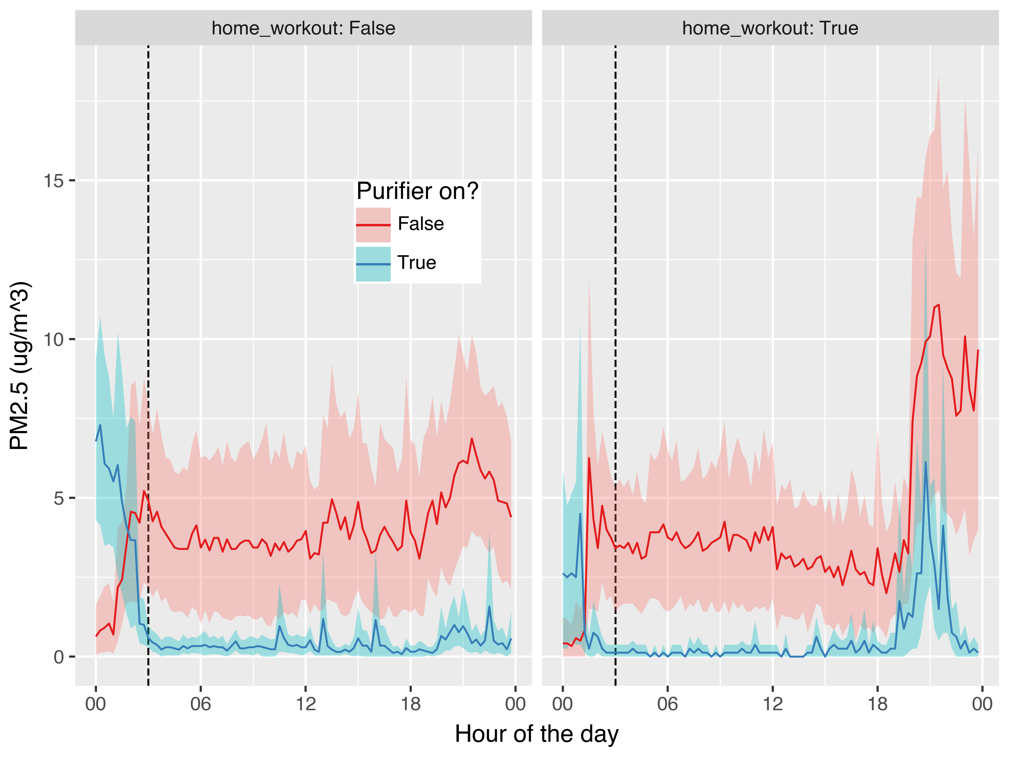
The average daily cycle confirms the washout of 3 hours is sufficient, and also shows elevated levels in the evening.
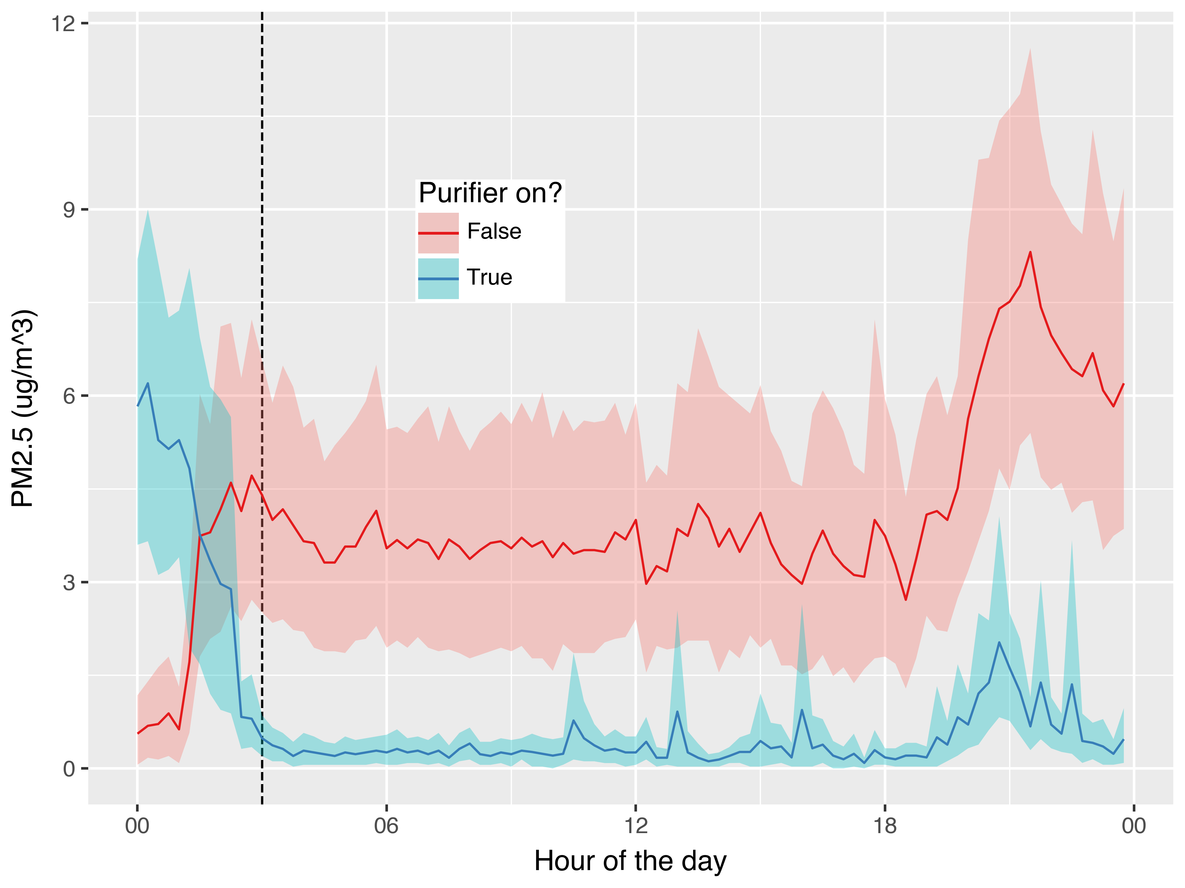
The evening peaks are almost all occurring on the days I did home workouts, during which I opened the windows to keep cool. Interestingly when the purifier is off, the pollution level increases and remains high. In contrast when the purifier is on, while the pollution level does increase, it also returns back to baseline after I’ve finished the workout. This is a kind of accidental experiment within the broader per-day experiment showing the action of the purifier!
Quantifying uncertainty via a Bayesian model
So far we’ve looked at the average levels for each condition, but how precise are these estimates?
When estimating the uncertainty we must account for the fact that the data are not independent but auto-correlated.
To solve this properly, we can use a Bayesian structured time series model.
For a single observation i that occurs within a specific phase instance j of type P, the reported integer outcome y_i is modeled as negative binomial:
\begin{aligned} y_i & \sim \text{NegativeBinomial}(\mu = \lambda_i, \phi) \\ \ln(\lambda_i) & = \mu + \gamma_j \cdot P_i + L_{i,j} \quad \text{(Full baseline)} \\ \end{aligned}
with three components that set the mean latent pollution level \lambda_i.
Because the model uses a log-link function, the relationship between the components is multiplicative on the outcome scale:
\lambda_i = \underbrace{\exp(\mu)}_{\text{Global Baseline}} \times \underbrace{\exp(\gamma_j \cdot P_i)}_{\text{Purifier Multiplier (per period)}} \times \underbrace{\exp(L_{i,j})}_{\text{Local Random Walk}}
This implies the air purifier removes a percentage of the pollution per unit time, rather than a fixed subtractive amount. For a high CADR air purifier, with low to moderate pollution, this seems reasonable.
The purifier effect \gamma_j is per-period and drawn from a shared hierarchical prior, allowing the effectiveness to vary across days while still pooling information. Because we encoded Phase B (Purifier ON) as P_i = -1, the remaining pollution fraction for period j is:
\text{Remaining Fraction}_j = \exp(-\gamma_j)
For example, a result of \gamma_j=3 corresponds to a remaining fraction of \exp(-3) = 0.05 i.e. a 95% reduction in particles.
The full model is:
\begin{aligned} y_i & \sim \text{NegativeBinomial}(\mu = \lambda_i, \phi) \\ \ln(\lambda_i) & = \mu + \gamma_j \cdot P_i + L_{i,j} \quad \text{(Full baseline)} \\ \\ \mu & \sim \text{Normal}(M_{\mu}, S_{\mu}^2) \quad \text{(Global Intercept)} \\ \\ P_i & = \begin{cases} 0 & \text{Phase A (Purifier OFF)} \\ -1 & \text{Phase B (Purifier ON)} \end{cases} \\ \\ \gamma_j & = \exp(\mu_{\log\gamma} + \sigma_{\gamma} \cdot \tilde{\gamma}_j) \quad \text{(Per-day purifier effect)} \\ \mu_{\log\gamma} & \sim \text{Normal}(M_{\log\gamma}, S_{\log\gamma}^2) \quad \text{(Mean log-purification effect)} \\ \sigma_{\gamma} & \sim \text{HalfNormal}(S_\gamma) \quad \text{(Between-day variability)} \\ \tilde{\gamma}_j & \sim \text{Normal}(0, 1) \quad \text{(Per-day raw offset, non-centred)} \\ \\ L_{i,j} & = \text{init}_j + \sum_{t=0}^{t_{i,j}} \epsilon_{t,j} \quad \text{(Local Random Walk)} \\ \text{init}_j & \sim \text{Normal}(0, \sigma_{\text{init}}^2) \quad \text{(Intercept for phase)} \\ \epsilon_{t,j} & \sim \text{Normal}(0, \sigma_{\text{level}}^2) \quad \text{(Random Walk jumps)} \\ \\ \phi & \sim \text{Gamma}(\mu_\phi = 5, \sigma_\phi = 5) \quad \text{(Overdispersion of NB)} \end{aligned}
where: \begin{aligned} M_{\mu} = \ln(5.0) \\ S_{\mu} = \ln(2) \\ M_{\log\gamma} = -1 \\ S_{\log\gamma} = 1 \\ S_\gamma = 0.5 \\ \sigma_{\text{init}} = 0.5 \\ \sigma_{\text{level}} = 0.25 \\ \mu_\phi = 5, \quad \sigma_\phi = 5 \end{aligned}
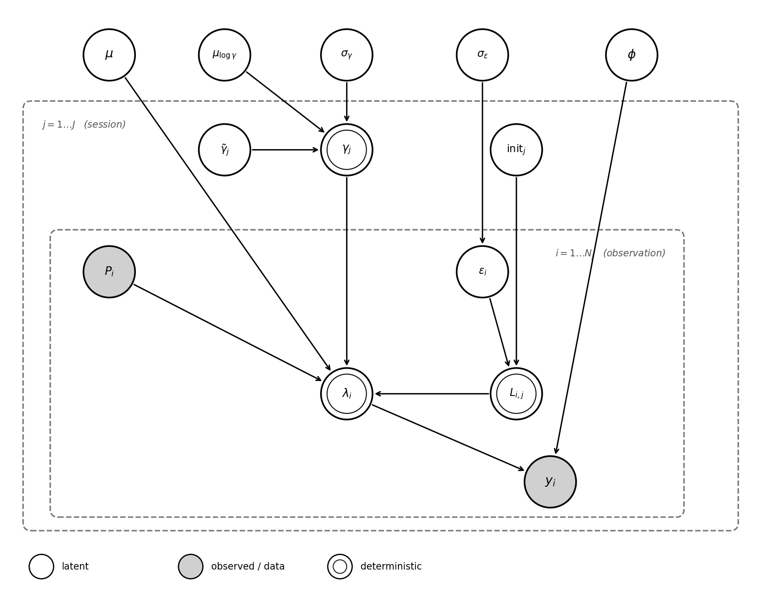
Components of the BSTS Model:
- y_i (Observed Outcome): The actual integer reading from the sensor.
- \lambda_i (Underlying Rate): The continuous latent PM2.5 concentration.
- \phi (Overdispersion): Controls the additional variance in the Negative Binomial distribution.
- P_i (Phase indicator): The phase indicator, which is 0 for Phase A (Purifier OFF) and -1 for Phase B (Purifier ON).
- \mu_{\log\gamma} (Mean log-effect): The global mean of the purifier effect on the log scale. The overall median efficiency is \exp(\mu_{\log\gamma}).
- \sigma_{\gamma} (Between-period SD): How much the purifier effect varies across periods on the log scale.
- \gamma_j (Per-period purifier effect): The treatment effect for period j, drawn hierarchically. Positivity is guaranteed by the log-normal parameterisation.
- \mu (Global Intercept): The baseline log-concentration of PM2.5, with a prior set so that the average is 5 ug/m^3 (slightly lower than the UK outdoor urban background).
- \text{init}_j (Session Initiation): The starting condition of the air at the exact minute the session began (\sigma_{\text{init}} = 0.5).
- \epsilon_{t,j} (Innovations): Random “jumps” in concentration between each measurement (every 15 minutes), with a standard deviation of \sigma_{\text{level}}.
- L_{i,j} (Hidden State): The resulting accumulated air quality trend for that specific timepoint.
That’s quite a lot, so here’s a visual representation of the model:
Modelling choices
The positivity of \gamma_j implies that the air purifier can not increase the amount of pollution (the \gamma_j \cdot P_i term becomes \exp(\gamma_j * -1) \in (0, 1)). I think this is reasonable though one could argue that by air circulation the purifier could kick up some settled particles and actually increase pollution levels.
The treatment effect \gamma_j is modelled using a hierarchical model to allow the efficiency to vary day by day, while still estimating a global latent mean. The hierarchical component uses a non-centered parameterisation to avoid the funnel geometry that the NUTS sampler can struggle to efficiently explore.
While the raw data I get from the device is in count/integer form, this is presumably due to some internal rounding by the device rather than it actually measuring counts (the units are ug/m3 after all). Hence NegativeBinomial is a misspecified likelihood from the perspective of representing the true data generating process - an interval likelihood would be more correct. However, practically, it’s simpler to use and accounts for the integer reality of the data and naturally allows for 0 values.
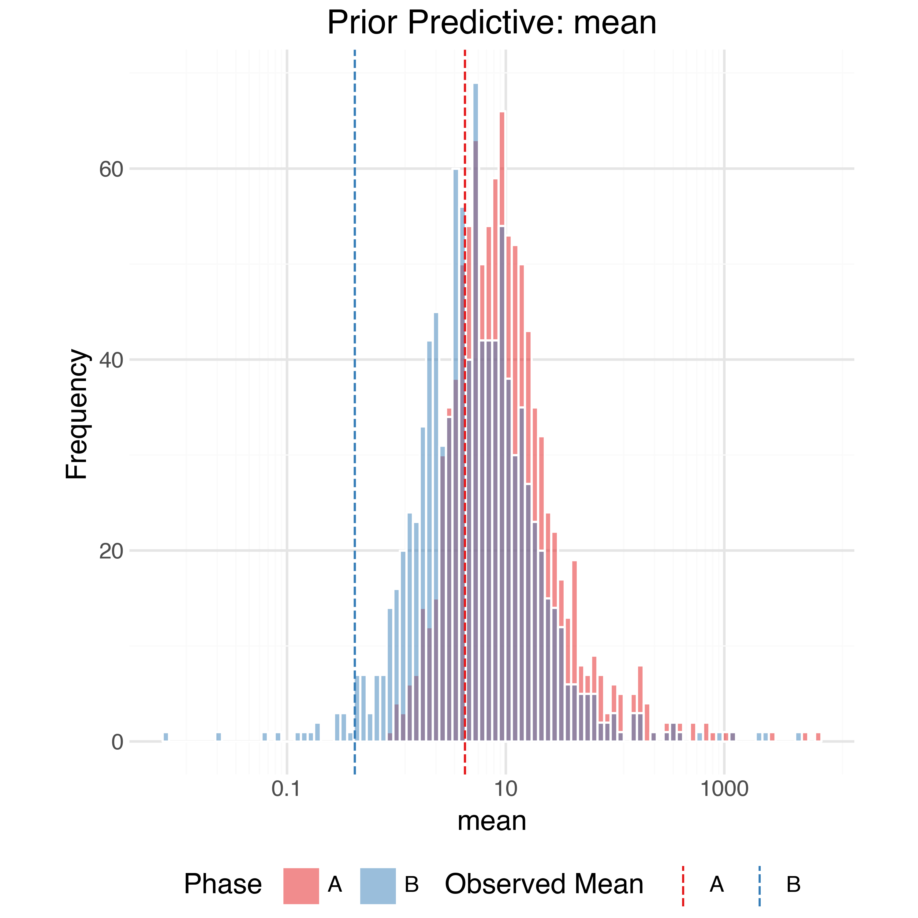
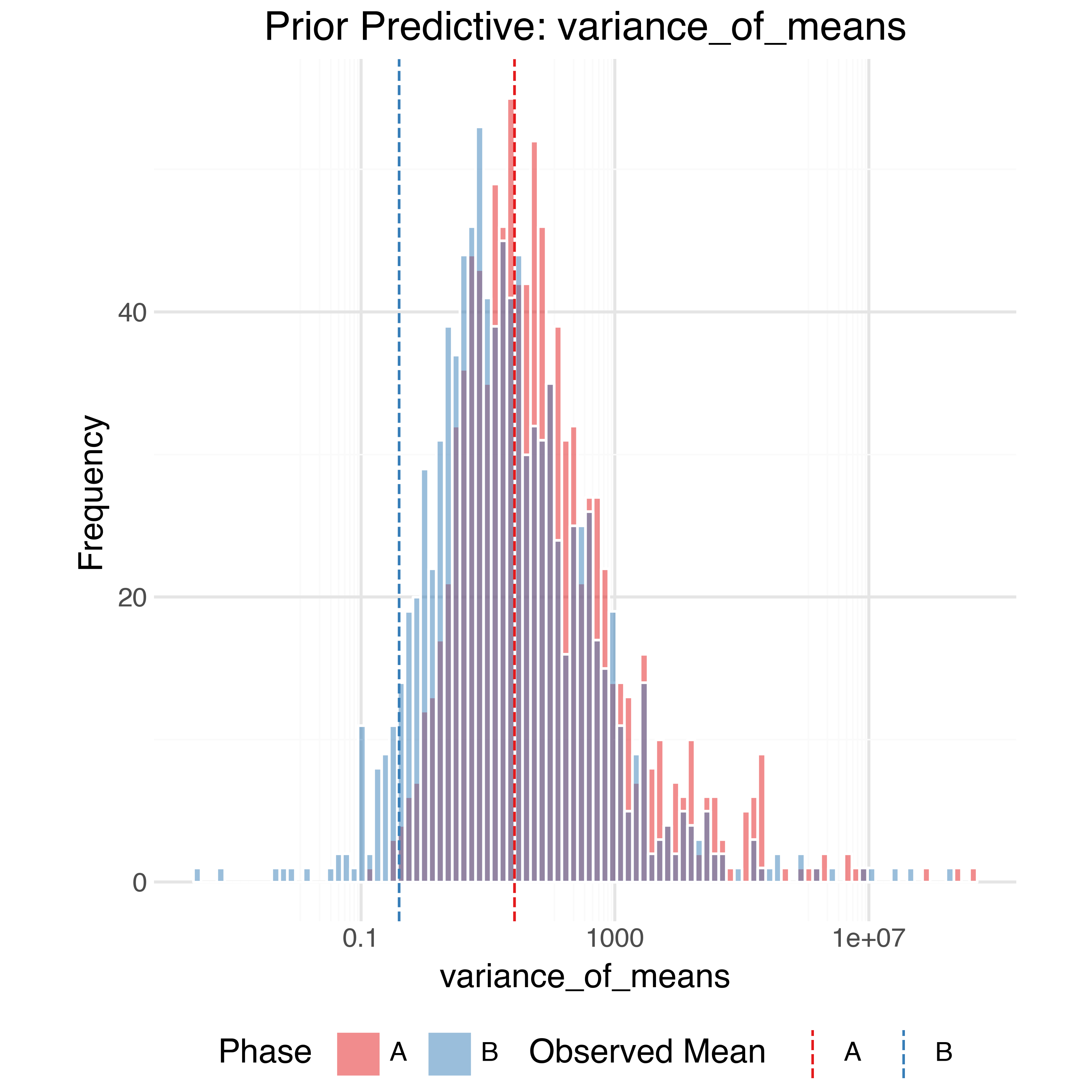
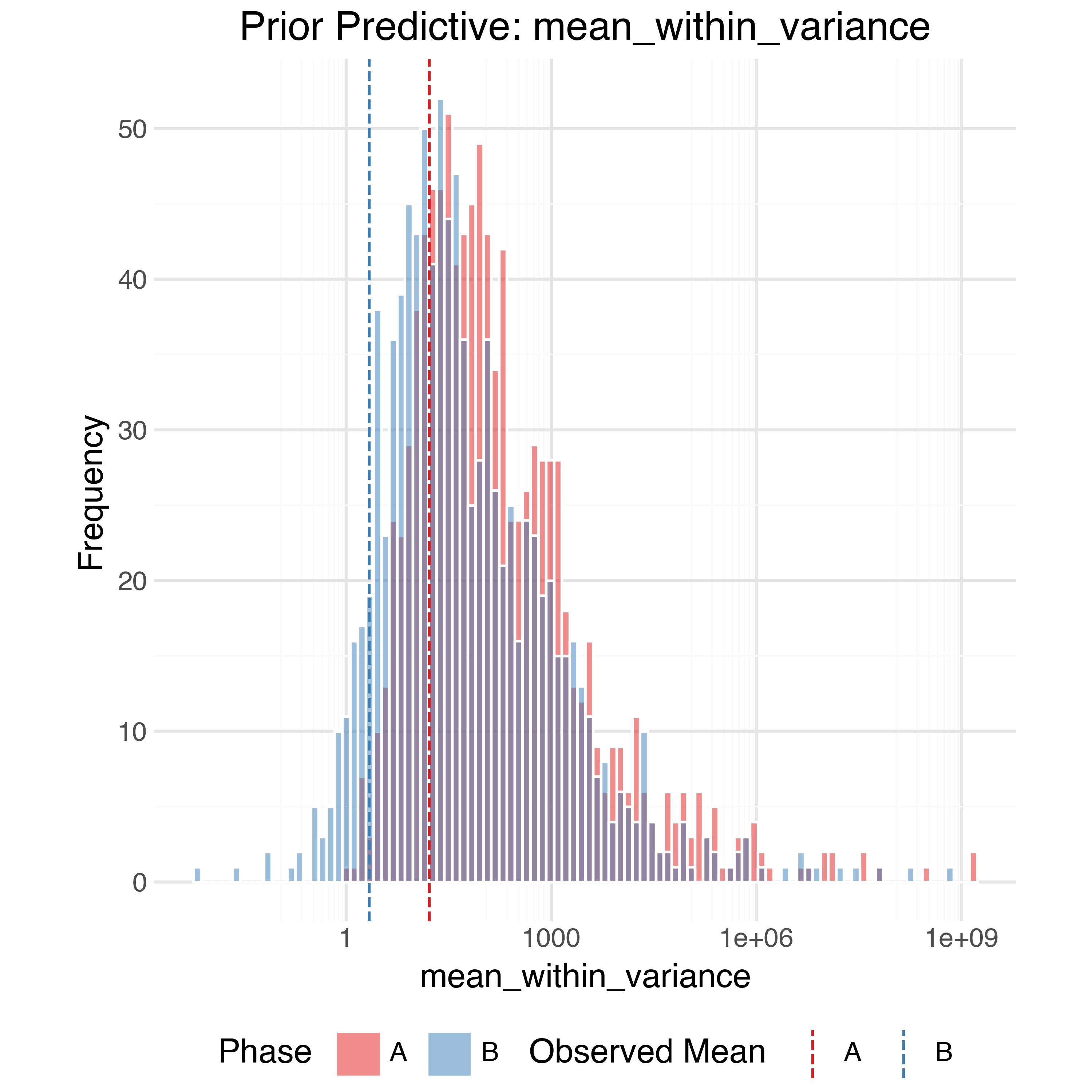
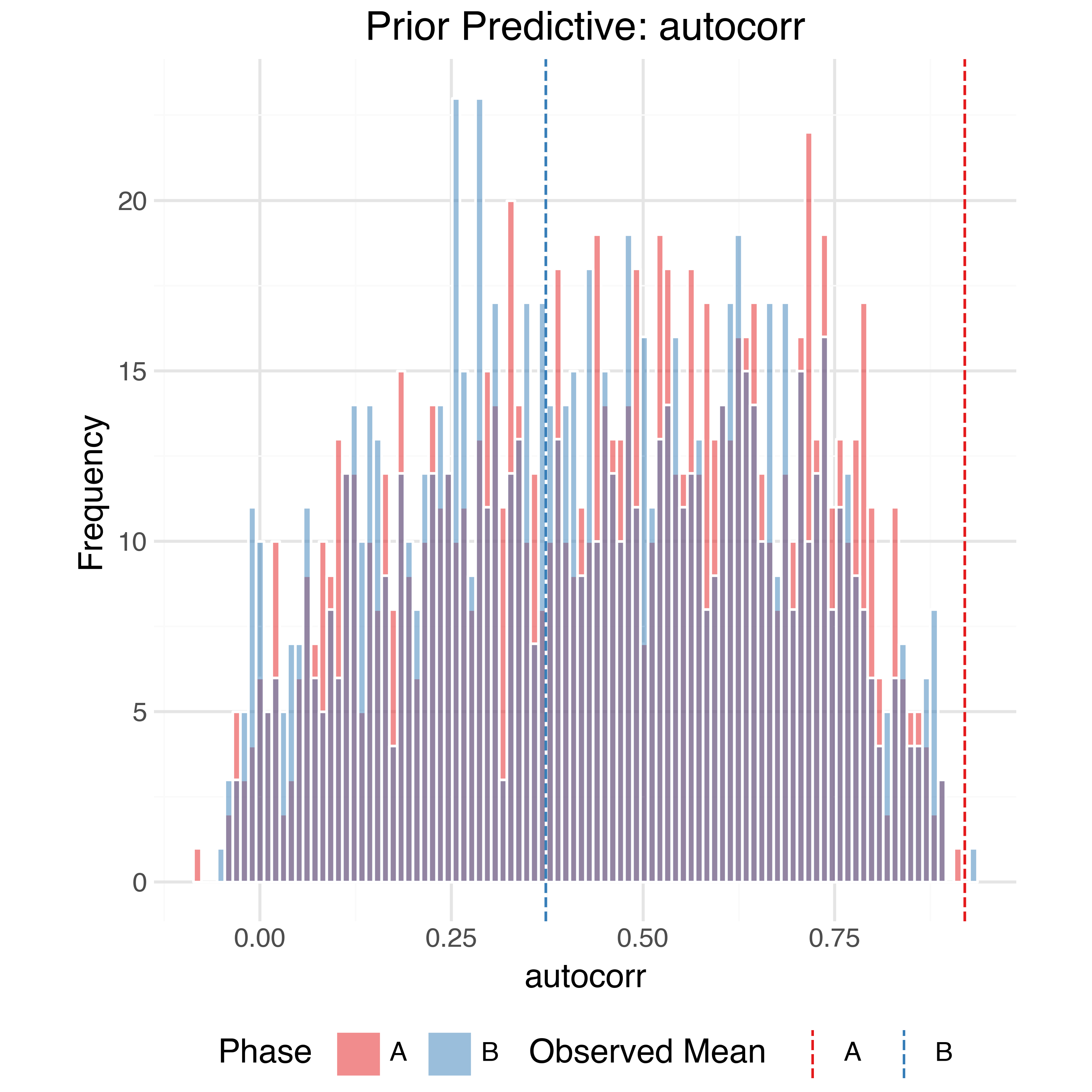
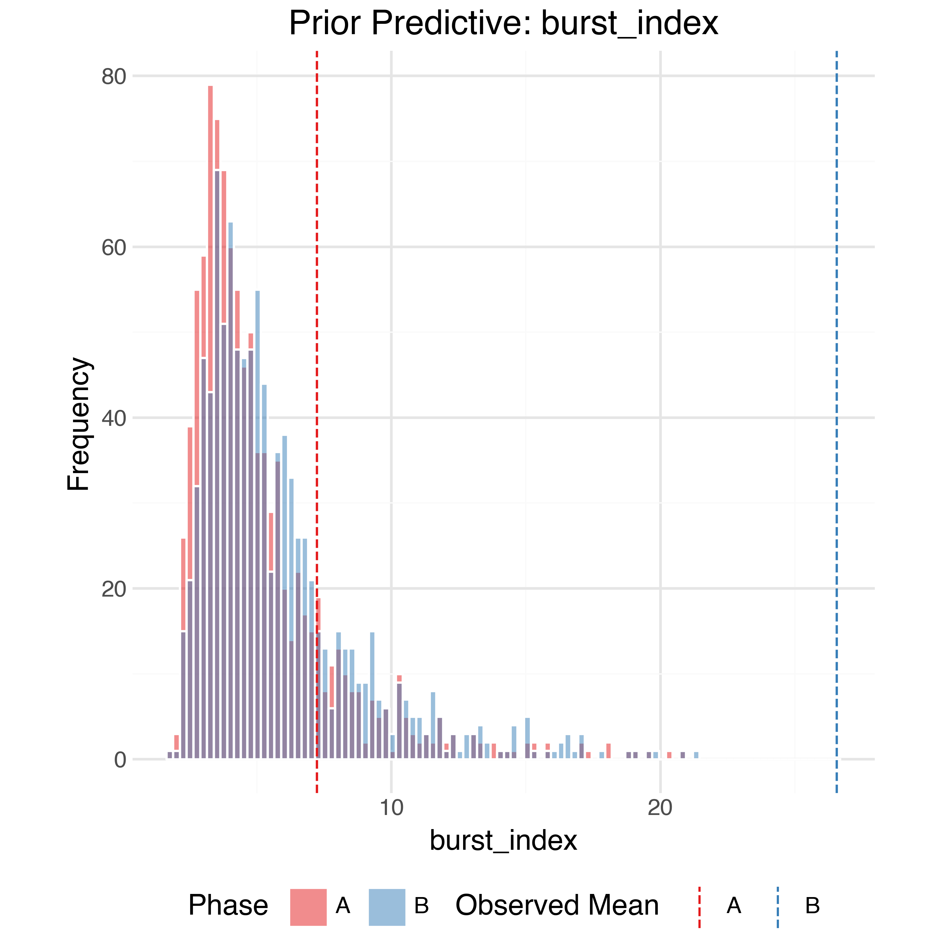
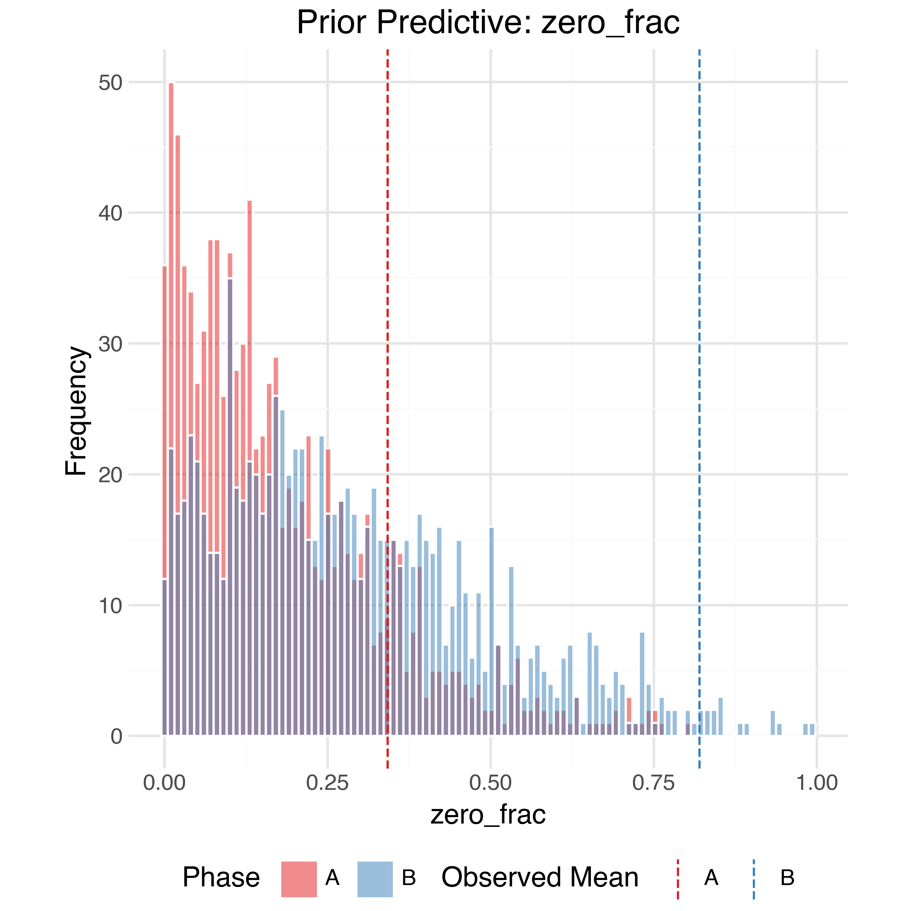
Prior pushforward distributions
One way to check the priors are reaonsable is looking at the distribution of some of the intermediate latent nodes of the model. These priors above imply the following distributions for the four top level model components:
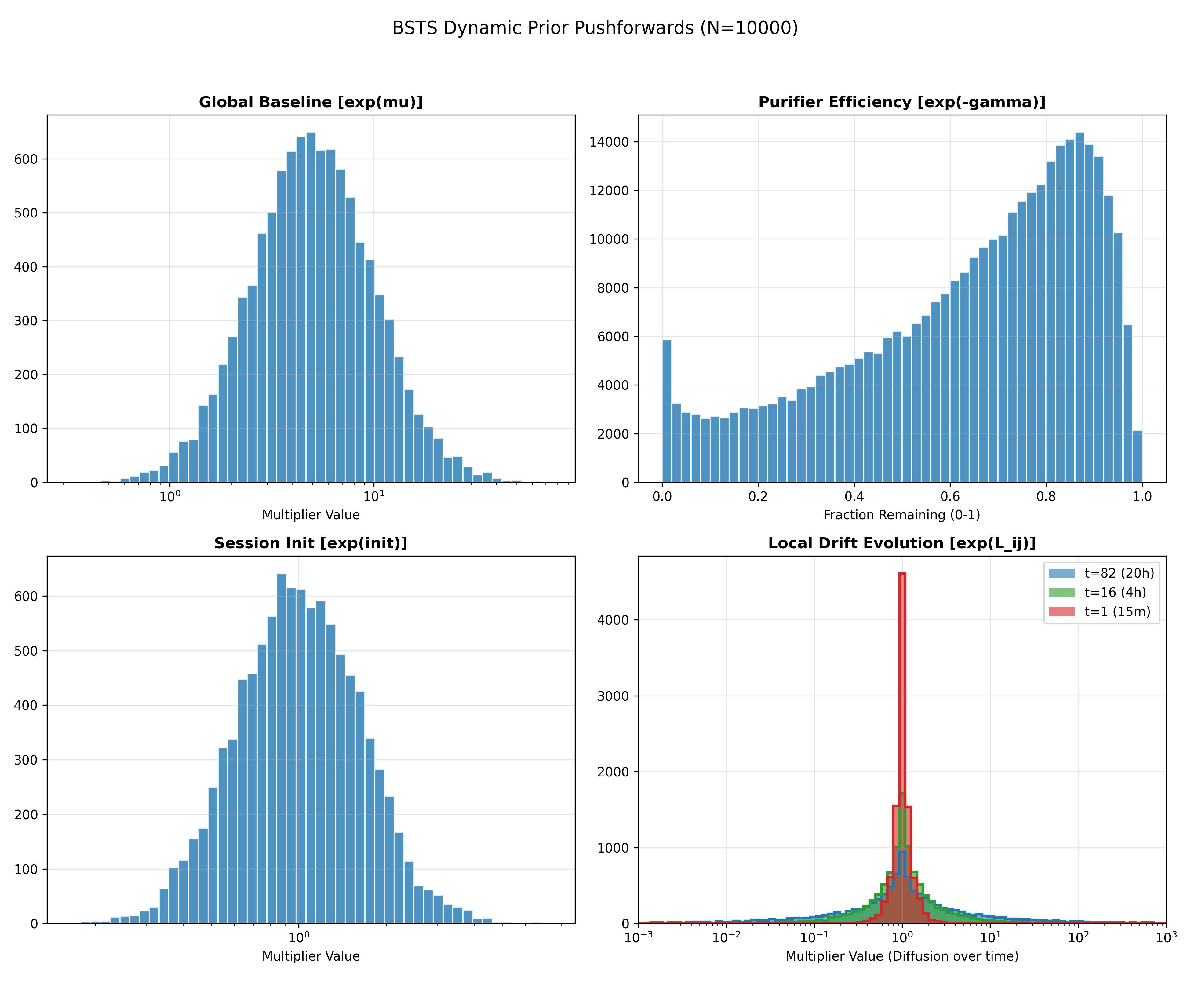
The prior on the effectiveness has most of its mass towards the higher range reflecting the manufacturers independently tested claims. However, there is substantial mass at lower values and even 0 representing the potential for much lower effectiveness given the shift in context of the current test and potential for marketing bias.
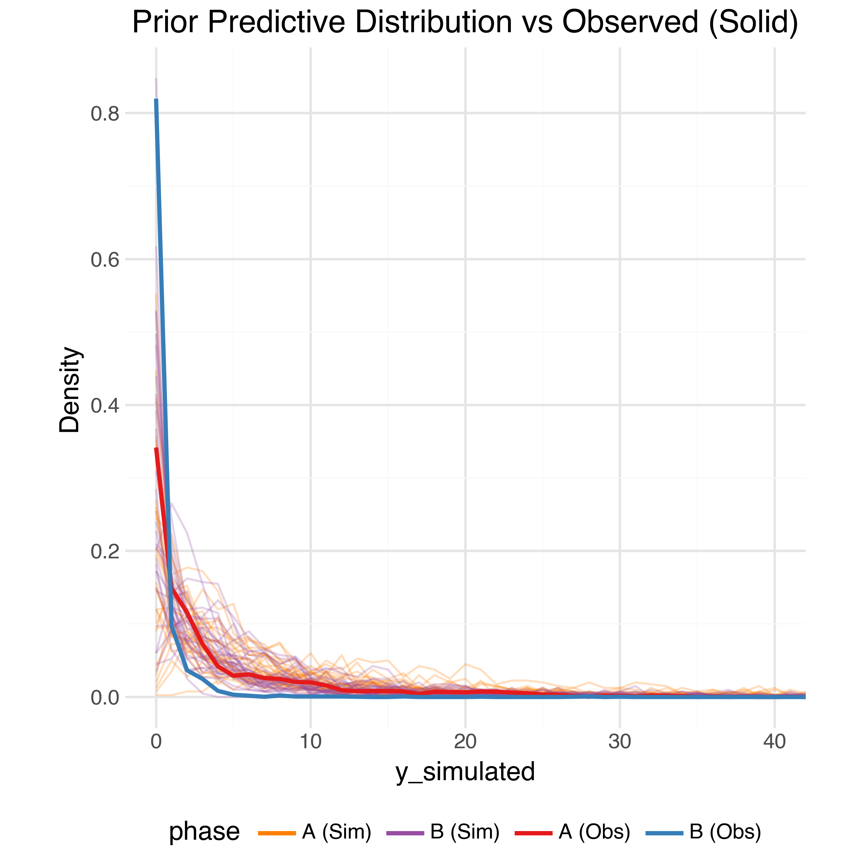
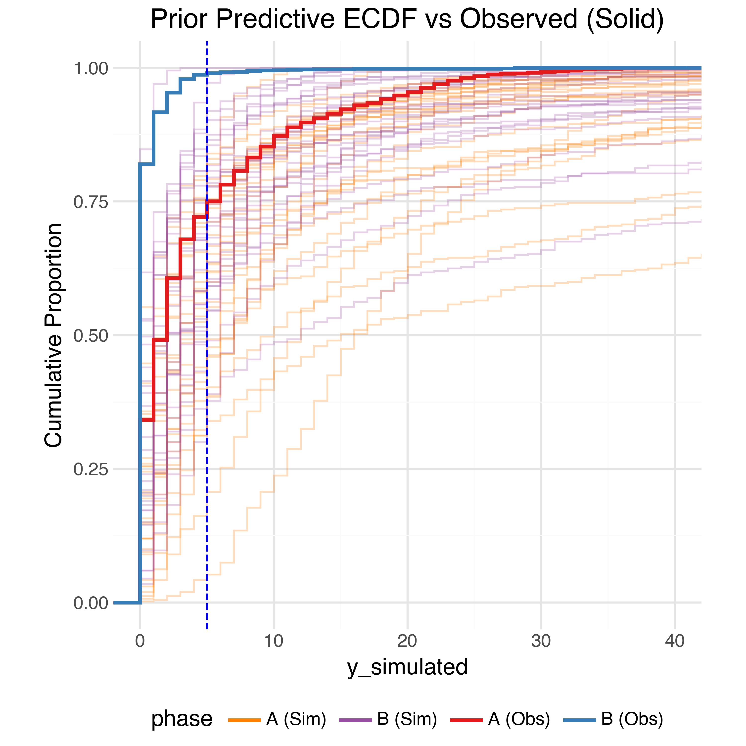
Prior predictive checks
In order to check the model is expressive enough to capture the data generating process while also not placing too much prior weight on unrealistic outcomes we can perform prior predictive checks. Using the priors defined above we can generate 1,000 simulated observed datasets from the model and compare (summaries of) them to the true observed data. The observed data should generally be within the bulk of the simulations.
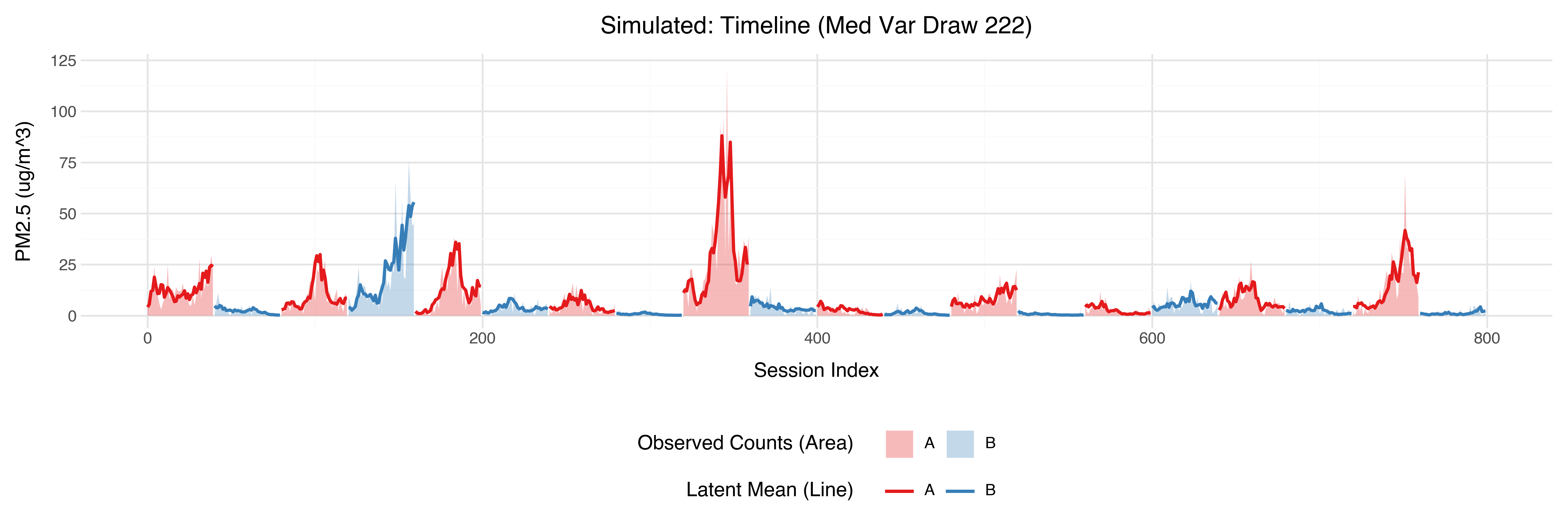
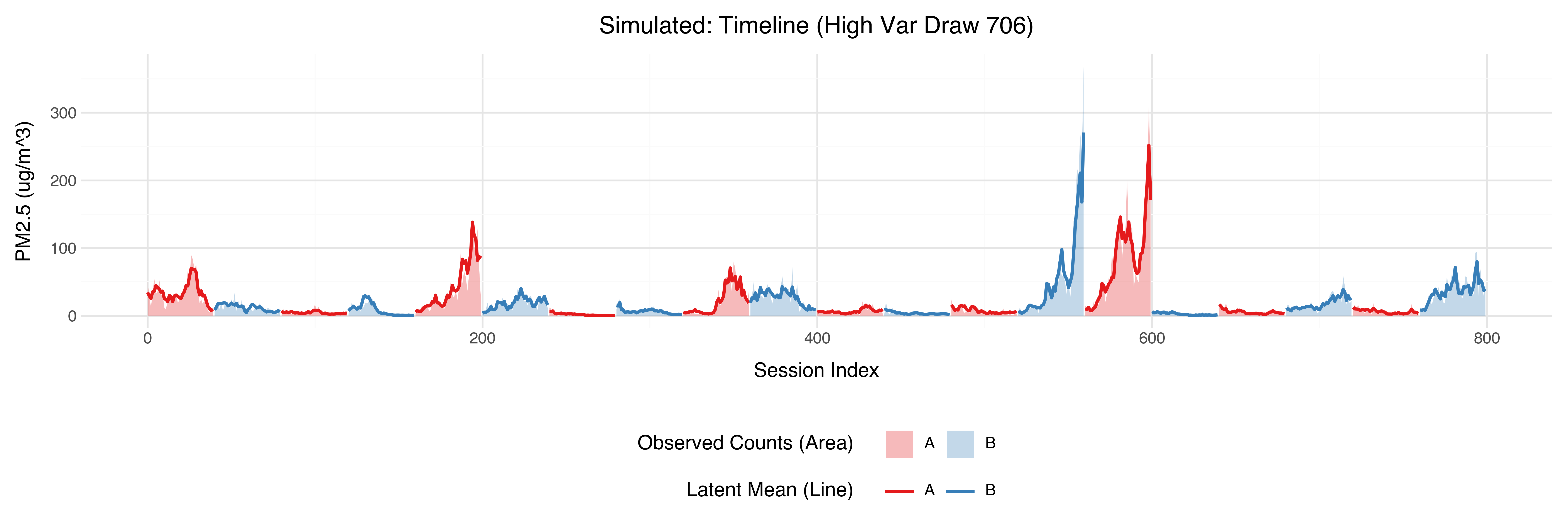
Sample Trajectories
At the raw data level, the simulated trajectories also seem reasonable:
Simulation based calibration checking
To ensure the model:
- has been faithfully implemented,
- can be fit using our inference engine (PyMC in this case),
- and that the resulting posterior distributions reflect the true uncertainty,
we can perform simulation based calibration (SBC). In SBC, we simulate datasets from the model with known parameters, fit the model to these datasets, and then check if the posterior distributions cover the true parameter values at the expected rate.
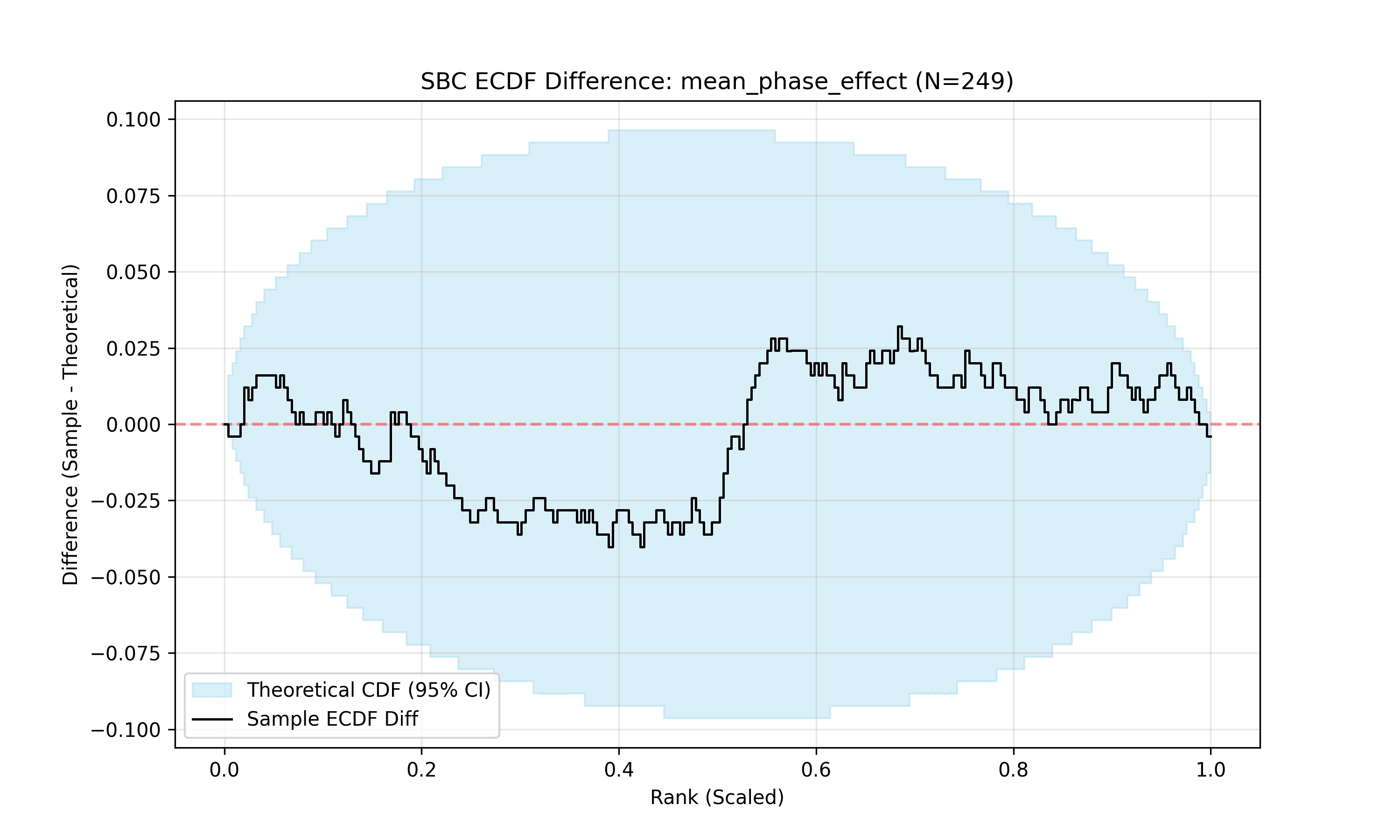
Across many simulations, the rank of the posterior parameter values should be uniform between 0 and 1.
The observed difference between the ECDF and the expected uniform distribution is within the range of expected differences (light blue band), suggesting the model is well calibrated.
Fitting the model
I fit the model using PyMC directly with the NUTS sampler (via the NumPyro JAX backend). The model was fit using 3 chains of 1000 iterations each, with a warm-up of 1000 iterations. The resulting summary statistics are shown below:
We can verify the sampler behaved well: R̂ is close to 1.0 for all parameters, ESS > 400, and there were no divergent transitions.
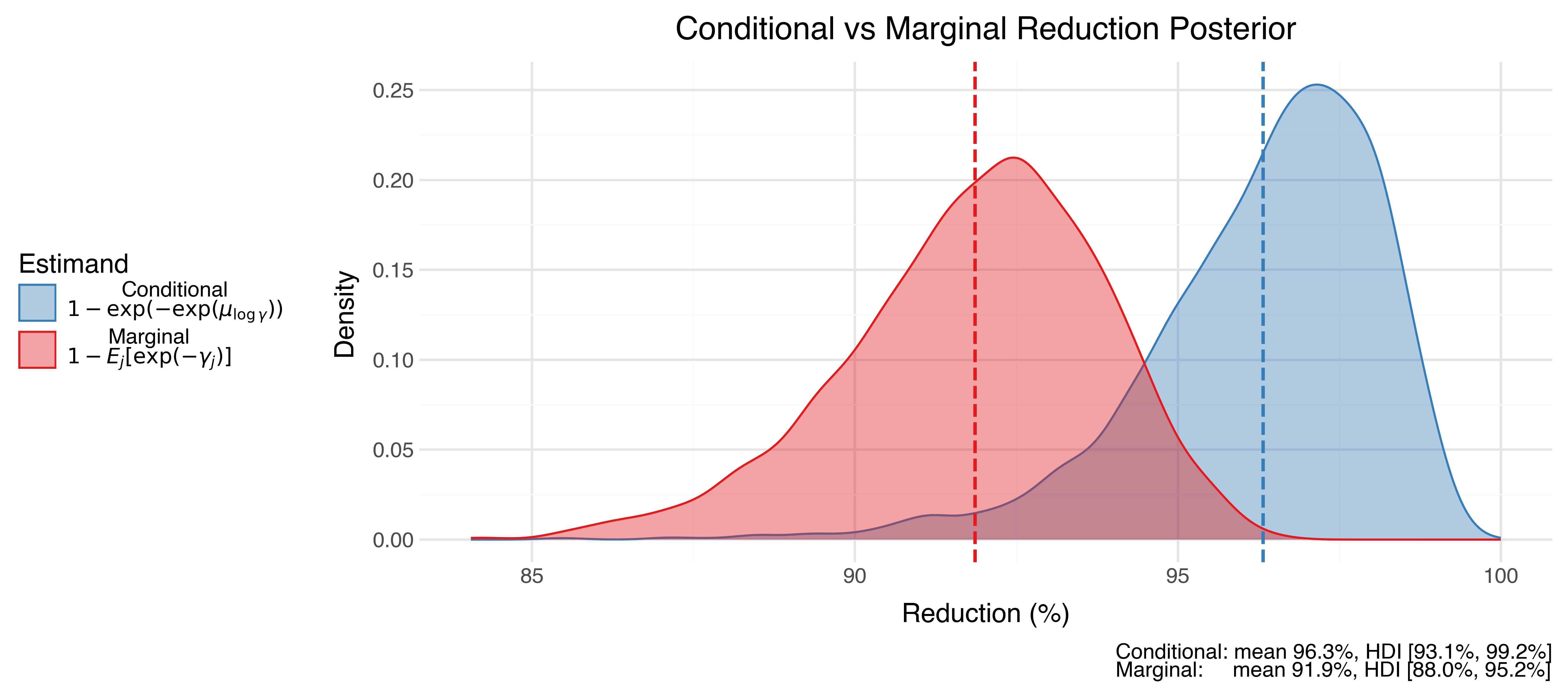
The global mean treatment effect (mean_phase_effect = \exp(\mu_{\log\gamma})) is estimated to be 3.4, which corresponds to a 96.3% reduction in PM2.5 levels with a 95% credible interval of [93%, 99%].
However, this treatment effect is the conditional reduction — the efficiency at the median day (i.e. setting \tilde{\gamma}_j = 0): 1 - \exp\!\bigl(-\exp(\mu_{\log\gamma})\bigr)
An alternative summary is the marginal reduction — the expected efficiency averaged across the distribution of days, approximately 91.9% [95% CI 88% to 95%]: 1 - E_j\!\bigl[\exp(-\gamma_j)\bigr]
Because \exp(-\gamma) is convex in \gamma, Jensen’s inequality guarantees the marginal reduction is always smaller than the conditional.
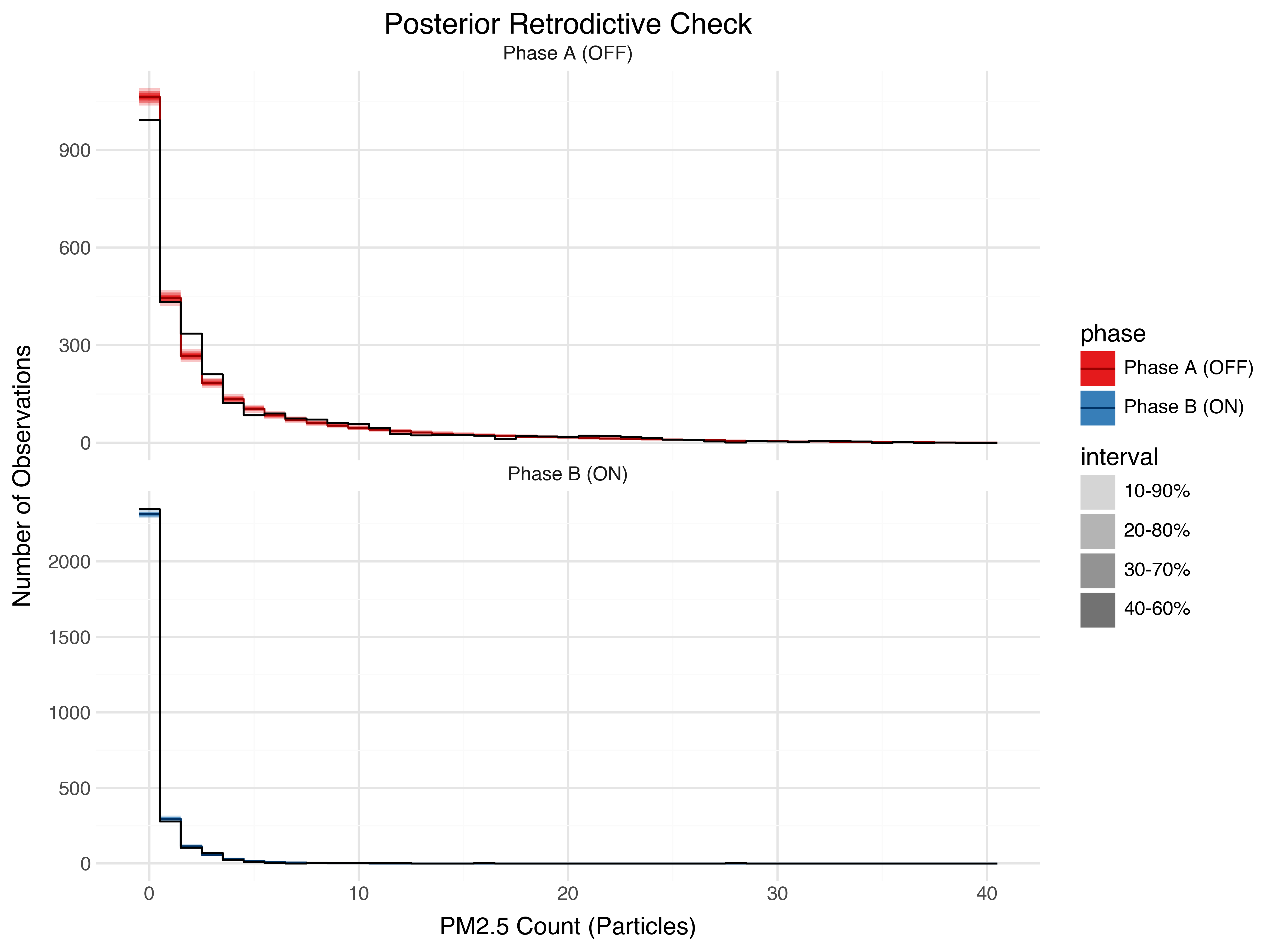
Posterior predictive checks
After we’ve fit the model, we can check its ability to reproduce the observed data by generating posterior predictive samples and comparing.
The overall distribution of counts fits reasonably well. 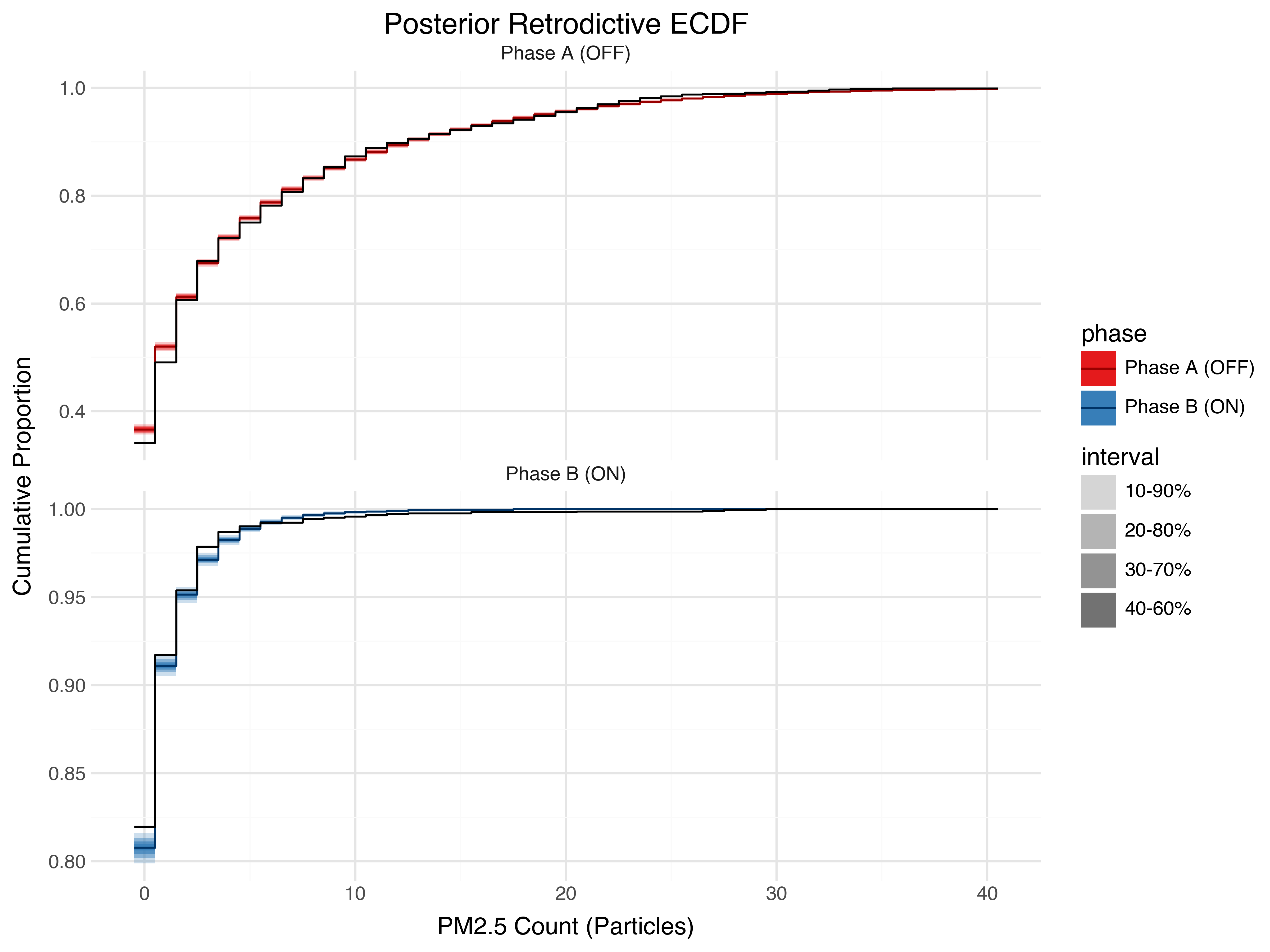
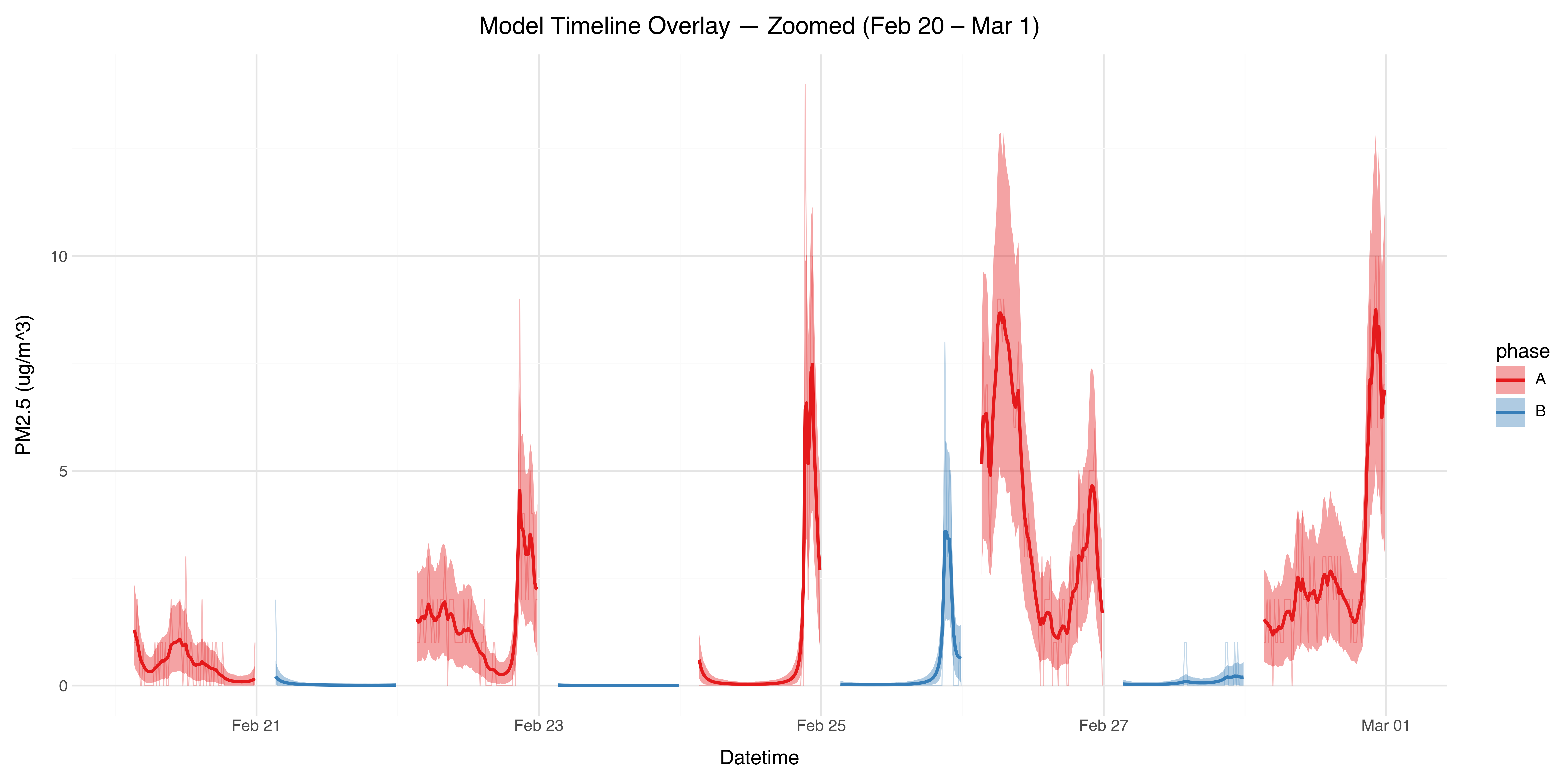
The daily fluctuations are also well captured by the random walk.
Sensitivity to estimation method
While the model developed above accounts for uncertainty in the mean effectiveness due to the data, it rests on the modelling assumptions. To understand uncertainty due to those assumptions, we need to look at alternative approaches as sensitivity analyses.
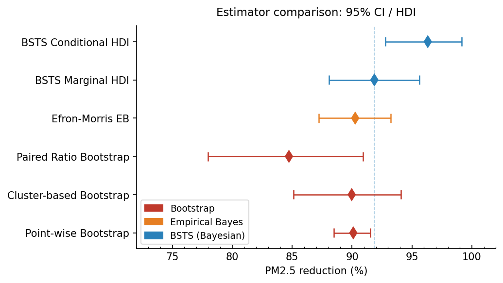
Point-wise Bootstrap
| Method | Mean (%) | Lower CI (%) | Upper CI (%) | Width (%) | |
|---|---|---|---|---|---|
| 0 | Point-wise Bootstrap | 90.11 | 88.56 | 91.56 | 3.0 |
\hat{\theta}_{PW} = 1 - \frac{\bar{B}_{\text{all}}}{\bar{A}_{\text{all}}}
Treats each 15-minute interval as an independent observation. Because consecutive readings are autocorrelated (pollution disperses slowly), this inflates the effective sample size and produces a spuriously narrow CI. Included here as a reference baseline only.
Cluster-based Bootstrap
| Method | Mean (%) | Lower CI (%) | Upper CI (%) | Width (%) | |
|---|---|---|---|---|---|
| 0 | Cluster-based Bootstrap | 90.05 | 85.42 | 94.02 | 8.6 |
\hat{\theta}_{CB} = 1 - \frac{\frac{1}{J}\sum_j \bar{B}_j}{\frac{1}{J}\sum_j \bar{A}_j}, \quad j = 1,\ldots,35
Resamples whole days as the natural experimental unit, correctly accounting for within-day autocorrelation. Takes the ratio of pooled period means, which gives more weight to high-pollution periods.
Paired Ratio Bootstrap
| Method | Mean (%) | Lower CI (%) | Upper CI (%) | Width (%) | |
|---|---|---|---|---|---|
| 0 | Paired Ratio Bootstrap | 84.73 | 78.32 | 90.94 | 12.62 |
\hat{\theta}_{PR} = 1 - \frac{1}{J}\sum_{j=1}^{J} \frac{\bar{B}_j}{\bar{A}_j}
Computes ratios per period before averaging, giving each period equal weight regardless of pollution level. Periods with near-zero Phase A concentrations (as low as 0.3 µg/m³) produce unreliable ratios that drag the mean down, explaining the lower estimate.
Efron-Morris Empirical Bayes
| Method | Mean (%) | Lower CI (%) | Upper CI (%) | Width (%) | |
|---|---|---|---|---|---|
| 0 | Efron-Morris EB | 90.26 | 87.22 | 93.22 | 6.0 |
\hat\theta_j^{EB} = \bar\theta + \frac{\hat\tau^2}{\hat\tau^2 + \sigma^2_j}\,(\hat\theta_j - \bar\theta)
The principled extension of James-Stein shrinkage to unequal variances. Each period’s estimate is shrunk toward the grand mean in proportion to its noise: \hat\tau^2 is estimated from the data as total between-period variance minus within-period sampling noise. Noisy periods (\sigma_j \approx 30\%) are shrunk nearly to the grand mean; typical periods (\sigma_j \approx 2\text{–}3\%) keep most of their raw estimate. The CI is narrower than the BSTS methods because \hat\tau^2 is treated as a fixed point estimate rather than a random variable with its own posterior uncertainty.
BSTS Marginal HDI
| Method | Mean (%) | Lower CI (%) | Upper CI (%) | Width (%) | |
|---|---|---|---|---|---|
| 0 | BSTS Marginal HDI | 91.86 | 88.09 | 95.63 | 7.54 |
\hat{\theta}_{marg} = \mathbb{E}_{\text{post}}\!\left[1 - \frac{1}{J}\sum_{j=1}^{J} e^{-\gamma_j}\right]
The fully Bayesian version of EB: the hierarchical prior \gamma_j \sim \text{Normal}(\mu_{\log\gamma}, \sigma^2_{\log\gamma}) infers the shrinkage strength \sigma^2_{\log\gamma} from the data, propagating its uncertainty into the credible interval. Averages the treatment effect over the full distribution of period-level effects. The cluster bootstrap CI is wider than the BSTS Marginal HDI because partial pooling borrows strength across all 35 periods, reducing uncertainty beyond what resampling alone achieves. Because this is a latent variable model, it can seperate noise and pollution spikes from the underlying mean, unlike the bootstrap which treats all observations as part of the signal.
BSTS Conditional HDI
| Method | Mean (%) | Lower CI (%) | Upper CI (%) | Width (%) | |
|---|---|---|---|---|---|
| 0 | BSTS Conditional HDI | 96.32 | 92.8 | 99.17 | 6.37 |
\hat{\theta}_{cond} = \mathbb{E}_{\text{post}}\!\left[1 - e^{-\mu_{PE}}\right]
Evaluates the treatment effect at the median day — the shared hyperparameter \mu_{\log\gamma} with no additional period-level deviation. Because 1-e^{-\gamma} is concave in \gamma, Jensen’s inequality guarantees \hat{\theta}_{cond} > \hat{\theta}_{marg}: evaluating the reduction at the average \gamma always exceeds averaging the reduction over a spread of \gamma_j values.
Counterfactual prediction for causal inference
One benefit of having a generative model is that we can do some causal inference, and simulate a Counterfactual for a specific day, what would happen if the air purifier stayed off?
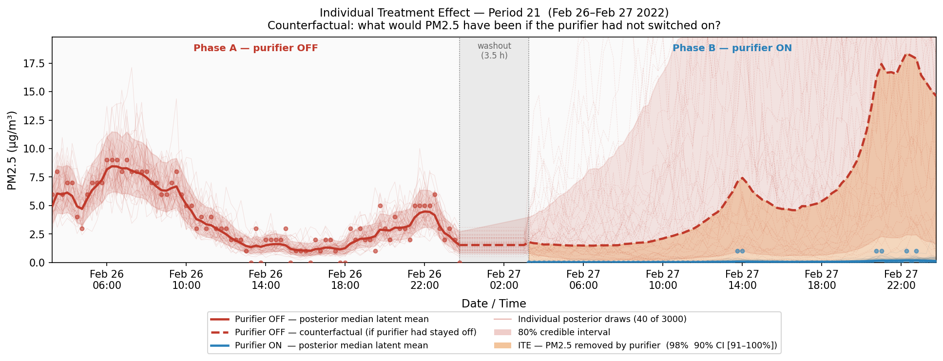
The orange band (difference between the counterfactual and the actual latent mean) shows the individual treatment effect (ITE) - the estimated reduction the air purifier had during this day.
Extension: modelling the workout spike with Gaussian processes
In the exploratory analysis I noted that the evening spike in pollution correlated with which day I did a home workout. This creates a nice experiment-witin-the-experiment. Instead of turning the purifier on and off, this turned a pollution source on and off. And because it’s a within day event, the counfounders are different to the main phase test. If the purifier was working effectively, we would expect pollution levels to reduce faster when the windows were closed compared to days when the purifier was not turned on.
To model this within day effect, I’m adding a Gaussian process to the log-rate:
- f_{\text{workout}}(t) — a smooth spike shape shared across all workout days (both phases), capturing the typical rise-and-fall around the workout.
- f_{\Delta}(t) — an additive Phase B only correction, capturing how the purifier modifies that shape. If the purifier accelerates recovery, f_{\Delta} should bend downward after the spike.
The log-rate gains two terms (active only on the relevant observations):
\ln(\lambda_i) = \mu + \gamma_j \cdot P_i + L_{i,j} + \underbrace{f_{\text{workout}}(t_i)\, W_i}_{\text{shared spike}} + \underbrace{f_{\Delta}(t_i)\, W_i \, B_i}_{\text{Phase-B correction}}
where W_i \in \{0,1\} indicates a workout day and B_i \in \{0,1\} indicates Phase B (purifier on). Each GP is given an ExpQuad covariance with its own lengthscale and amplitude:
\begin{aligned} f_{\text{workout}} & \sim \mathcal{GP}\!\bigl(0,\; \eta_{w}^2\, k_{\text{ExpQuad}}(t, t'; \ell_{w})\bigr) \\ f_{\Delta} & \sim \mathcal{GP}\!\bigl(0,\; \eta_{\Delta}^2\, k_{\text{ExpQuad}}(t, t'; \ell_{\Delta})\bigr) \\ \ell_{w}, \ell_{\Delta} & \sim \text{InverseGamma}(3, 0.2) \quad \text{(median} \approx 0.1 \text{ days} \approx 2.5\text{h)} \\ \eta_{w} & \sim \text{HalfNormal}(0.8) \\ \eta_{\Delta} & \sim \text{HalfNormal}(0.5) \quad \text{(tighter: a correction, not a full spike)} \end{aligned}
After fitting this model, the posterior trajectories indeed follow our expectation: a pollution spike occurs in both phases, but on days the purifier is active it returns to baseline, whereas on days the purifier is off it remains elevated.
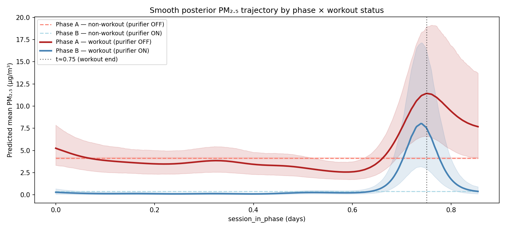
This is a satisfying confirmation of the purifier effectiveness, that is somewhat orthogonal to the main test.
Whether the health benefits outweigh the cost of purchasing and running the purifier (upfront, space, electric, and replacement filters) is another question.
However based on this experiment I’m more confident that, even in a real world scenario, the purifier is highly effective (86 - 95%) though not quite as effective as claimed based on the lab tests (99%).